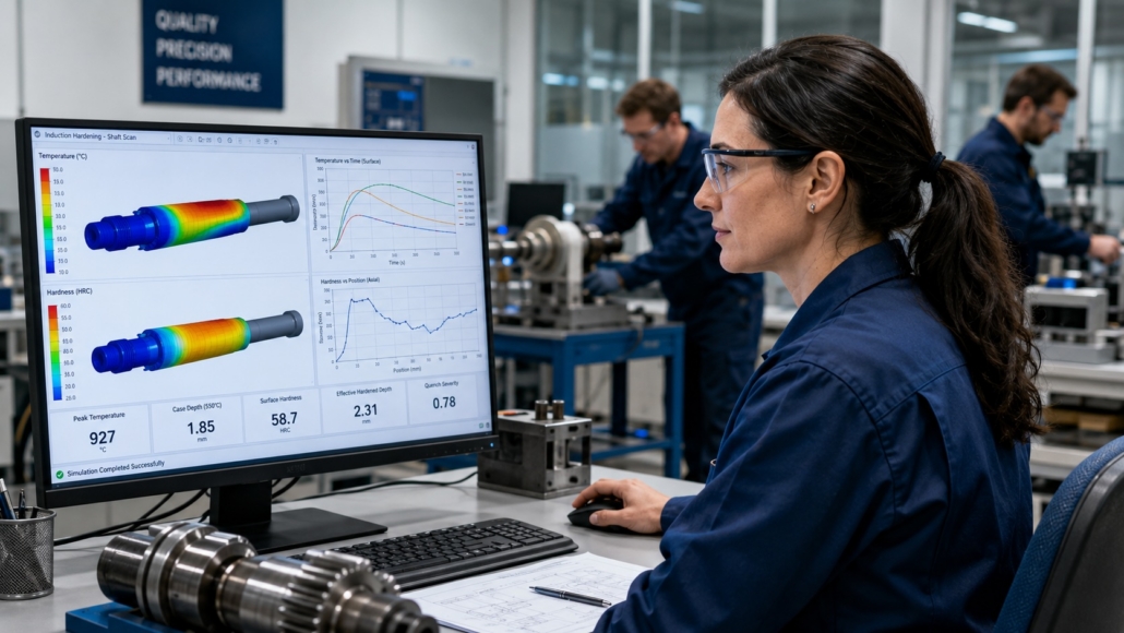
Induction hardening validation: how to compare simulation results with lab tests - CENOS : Simulation Software : Induction Heating : Radio Frequency : Wireless Charging

Validation is not about proving a simulation is perfect. It is about checking whether it is close enough to help you make good engineering decisions.

This is where comparison often gets messy. Teams look at one final simulation image, place it next to one lab result, and decide the model works. But that only shows the end result. It does not show whether the process behind it was modeled the right way.

A better approach is to compare the process step by step. First check the setup, the motion, heating and cooling, then check the results, hardening profile. When these parts line up, the final result means much more.

In this article, we use the CENOS splined shaft scanning example and the SMS Elotherm case to show how this comparison works in practice.

The main idea is simple: do not start with the final hardening pattern. First compare the things that create it.

What engineers usually compare first

The first thing engineers might compare is case depth or one hardening cross-section. That is important, but it should not be the first step.

First, make sure the simulation and lab setup match in these points:

part geometry and any simplifications
inductor geometry and number of coil turns
motion path and scanning speed
cooling position and cooling strength
input type: current, voltage, or power
time step settings
measurement point in the lab and evaluation point in the simulation

If one of these is wrong, the final hardening result can still look good while the model is wrong underneath. Simulation helps a lot, but it cannot fix a poor setup.

Quick setup checklist before comparing results

Before looking at temperature, case depth, or hardness profile, go through this short check:

is the part geometry the same as in the lab test?
were any small features removed or simplified in the model?
is the inductor geometry the same, including turns and spacing?
is the coil-to-part position the same?
is the scan direction the same?
is the scanning speed the same?
is the cooling position the same relative to the coil?
is the cooling delay the same?
is the electrical input defined the same way in both cases?
are you comparing the result at the same location and same time?

This checklist sounds basic, but it removes many false comparisons early.

The shaft case setup

This video shows the physical side of shaft scanning hardening. This particular video is an example to illustrate the physical prototype in the lab environment. For the simulation example, we will use another shaft design.

The inductor travels along the shaft, heating a narrow zone step by step, while cooling follows in a controlled way. The hardened result depends on this motion, not only on the final power setting.

Video: Example of shaft scanning hardening in the lab or production environment. The moving heating zone and cooling position are critical parts of the validation setup.

Video credit: YouTube channel of Heat Treating Corp

That is why a useful validation process starts with the setup. Before comparing hardness depth or one final cross-section, make sure the simulated case matches the real test conditions: part position, coil location, scan speed, heating time, and cooling layout. When these match, the result comparison becomes much more meaningful.

The shaft scanning case is a good validation example because the setup is concrete. CENOS shows a two-turn inductor with a flux concentrator, and one documented result is a hardening profile after 15 seconds of heating at 10 kHz, 6 kA, and 10 mm/s scanning speed.

Case study setup view from the shaft scanning example.

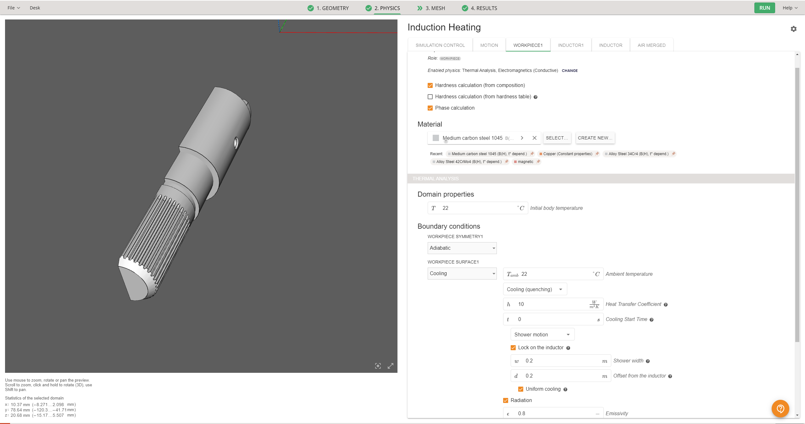
Physics setup view for the workpiece, including cooling settings.

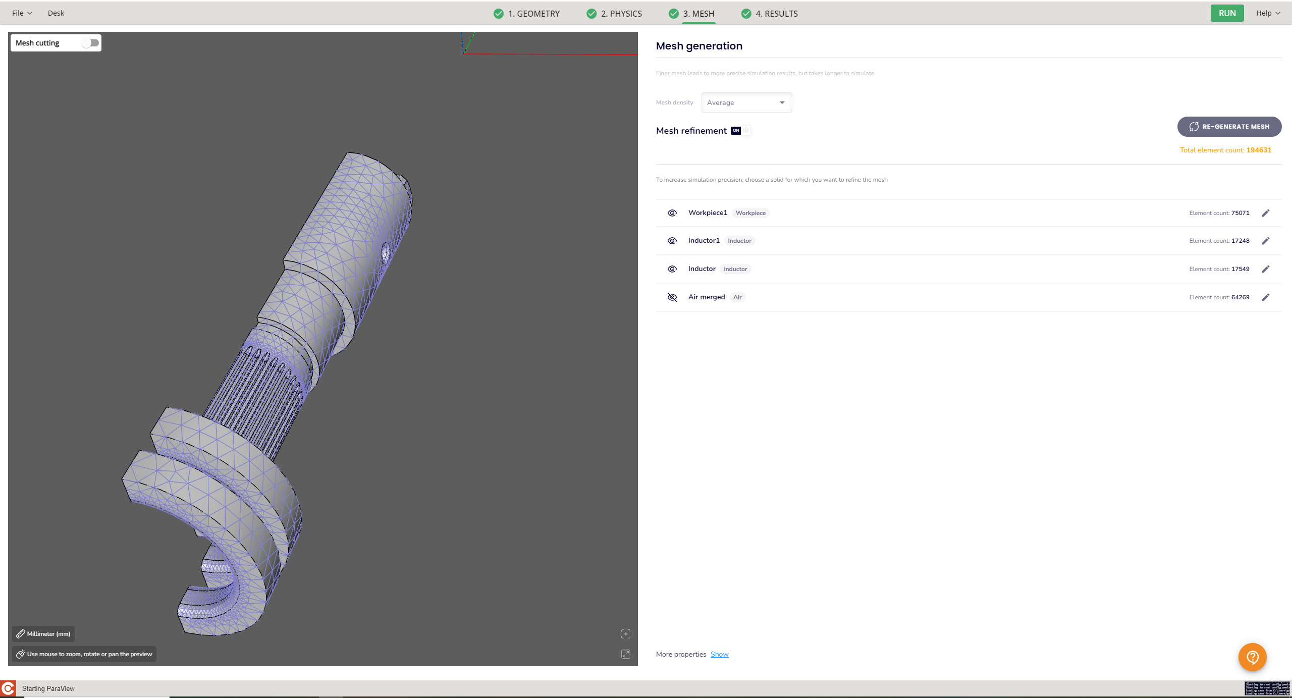
Mesh view of the shaft scanning model.

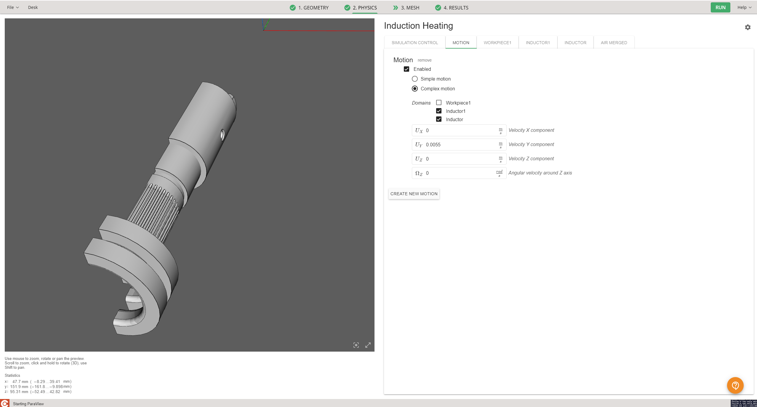
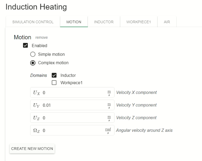
Motion setup for the scanning case.

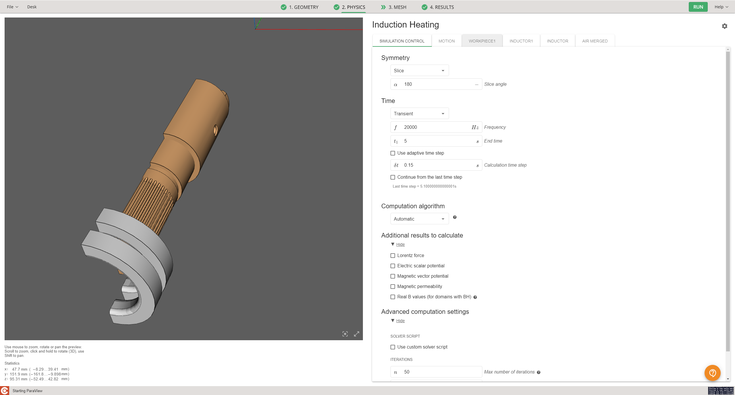
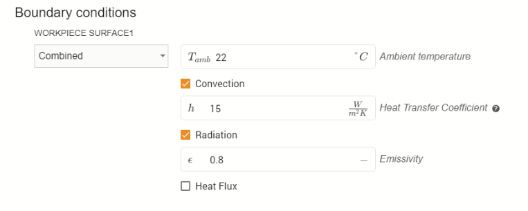
The splined shaft tutorial shows the same kind of setup logic in a more step-by-step way: transient simulation, a defined time step, assigned workpiece material, combined convection and radiation on the workpiece surface, current input on the inductor, and complex motion for the scan.

Geometry and simulation control view from the splined shaft tutorial.

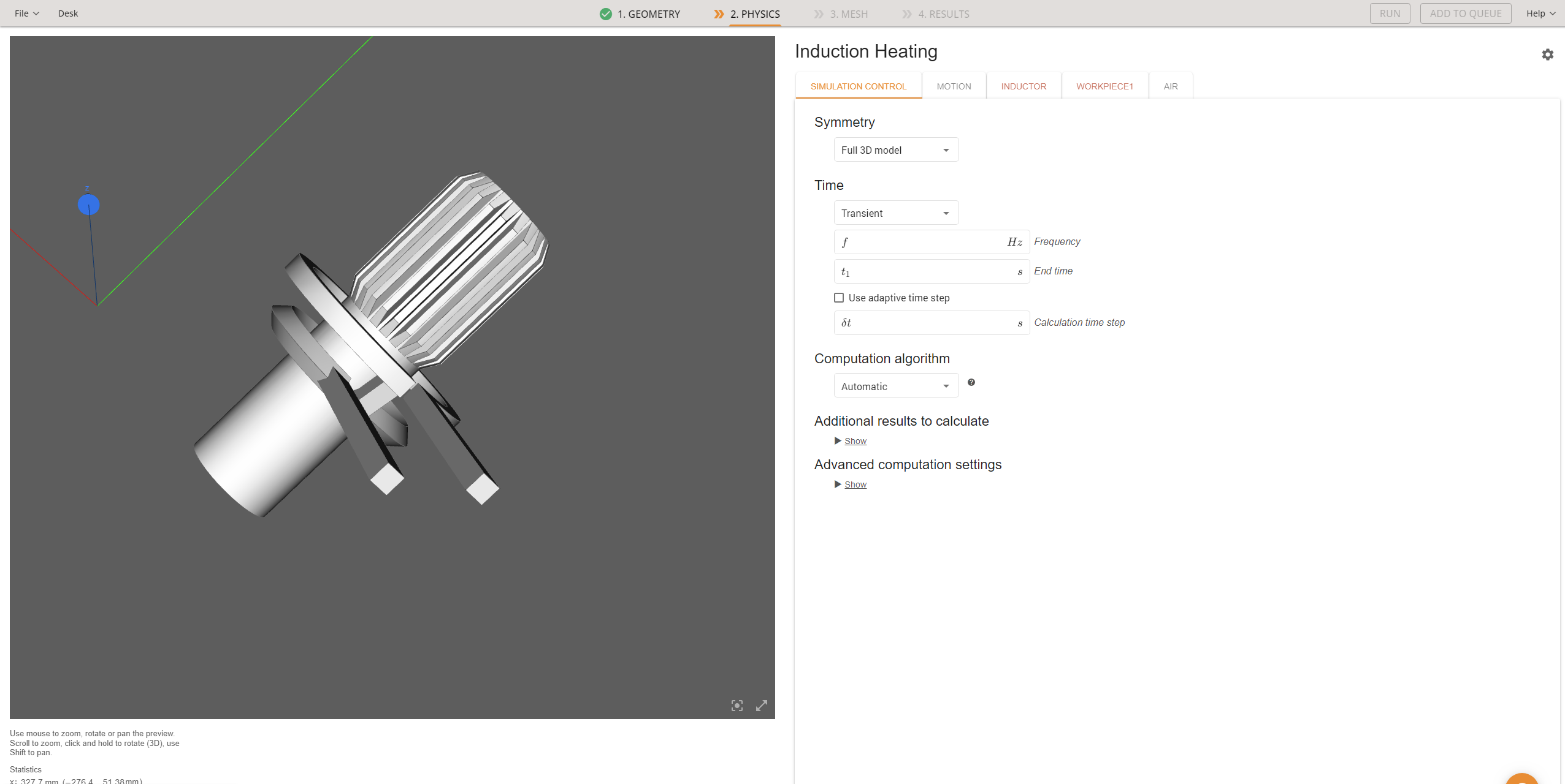
Simulation control: transient run with defined frequency, end time, and time step.

Splined shaft tutorial simulation control

Workpiece surface boundary conditions with convection and radiation.

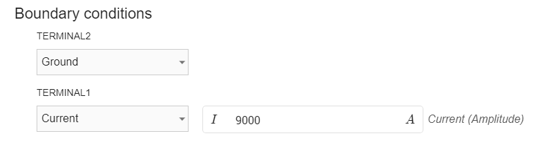
Splined shaft tutorial thermal boundary conditions

Inductor boundary conditions with current input.

Splined shaft tutorial inductor current input

Complex motion setup used for scanning.

Splined shaft tutorial motion definition

That is important in validation because the lab test must mirror those assumptions. Same part. Same coil. Same relative motion. Same cooling position. Same electrical input definition. Same evaluation time.

For a shaft scanning case, this is a useful setup checklist:

confirm shaft orientation
confirm scan start point and end point
confirm scan length
confirm scan speed
confirm whether there is any dwell before scanning
confirm coil position relative to the shaft surface
confirm quench position relative to the heating zone
confirm frequency
confirm current, voltage, or power input definition
confirm heating time and total simulation time
confirm time step size for the moving scan
confirm material and hardening assumptions

If these points are not aligned, it is too early to judge whether the simulation matches the lab.

Which outputs are most important

For induction hardening validation, four result groups are most important.

1. Temperature field

This tells you whether the heat goes where you think it goes. In the shaft case, the temperature gradient and the cooling transition show whether heating and quenching are positioned correctly relative to the moving part.

Temperature field at the end of the simulation.

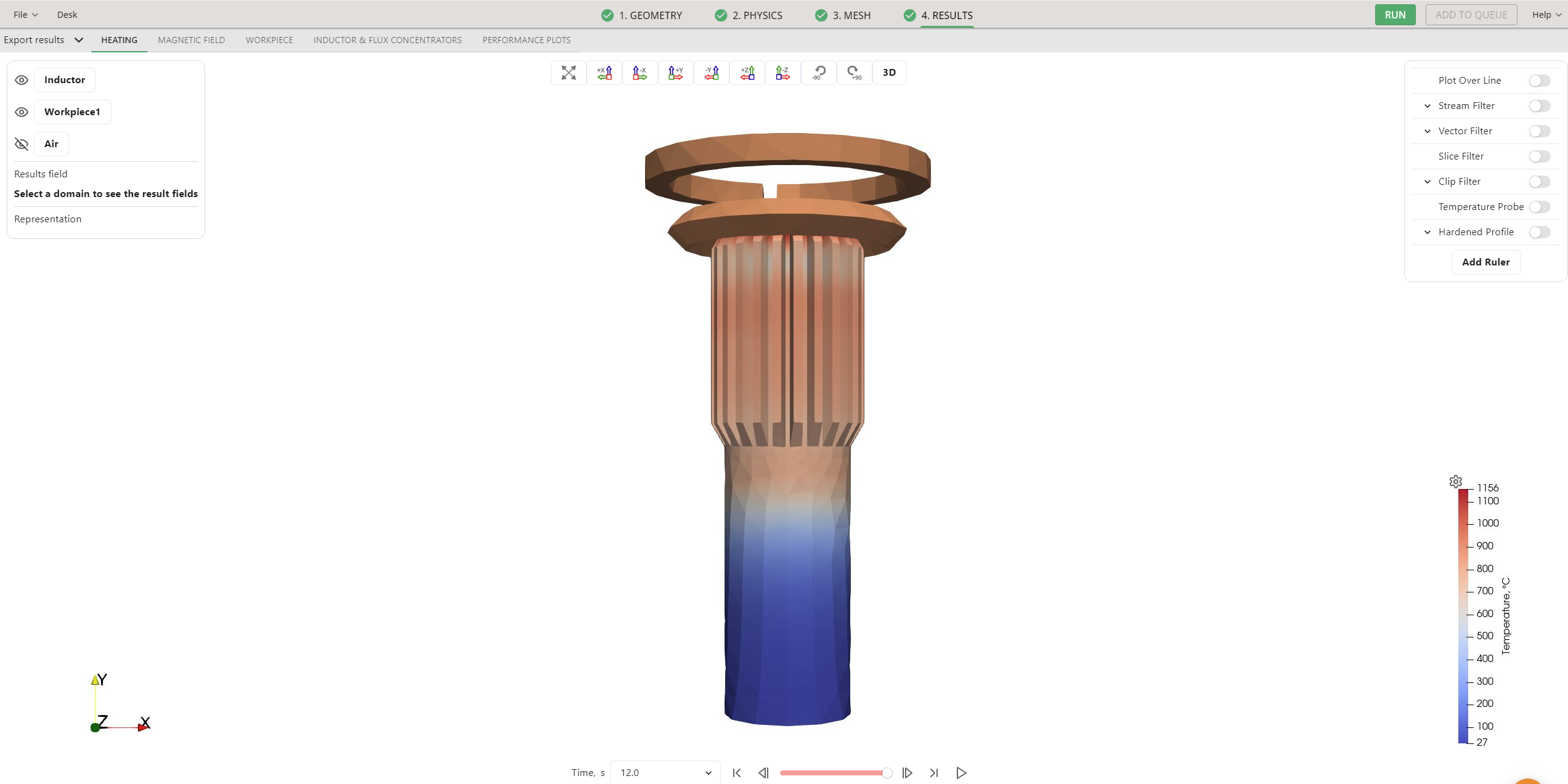
Temperature progression in the shaft scanning case.

In the lab, compare this against measured temperatures only at positions and times you can define clearly. Use known reference points and known timestamps.

What to check in temperature comparison

Is the hot zone in the same position?
Does the hot zone move the same way during the scan?
Is the peak temperature in the expected range?
Does cooling begin at the correct point?
Are you comparing temperature at the same location in lab and simulation?
Are you comparing at the same moment in time?

If the temperature story does not match, the hardening result will usually not match either.

2. Hardened zone

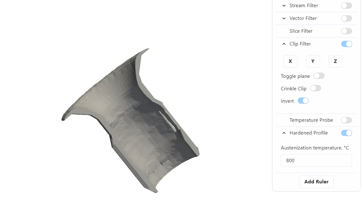
The hardened zone is the result most people want to jump to. Use it, but use it after the setup and temperature story make sense. The hardened profile filter in the CENOS Results Viewer shows where the chosen austenitization threshold has been reached.

Hardened profile view in CENOS Results Viewer.

Measured hardened zone view from the shaft example.

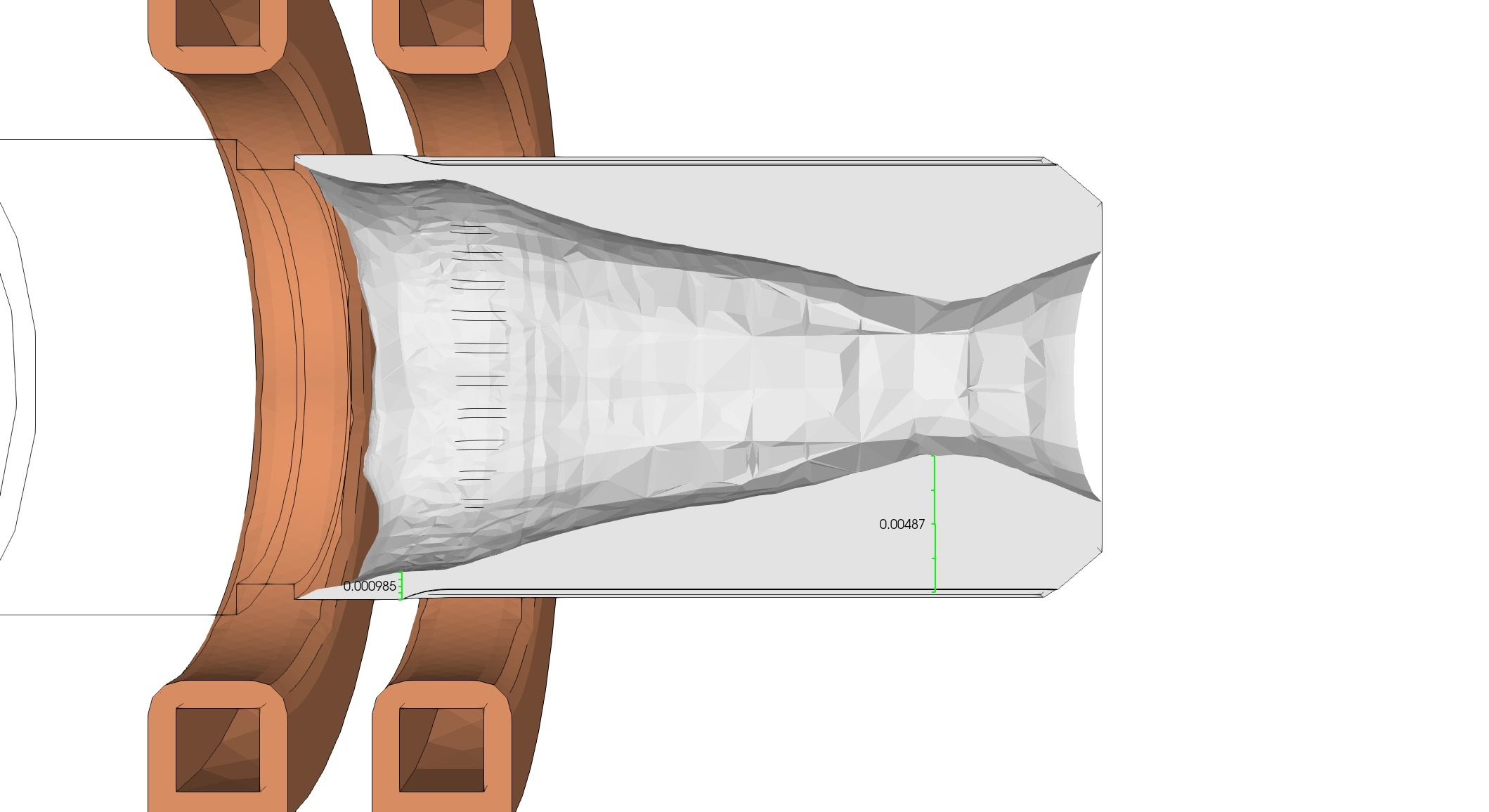
In the lab, compare the zone shape, its start and stop positions, and its depth at fixed reference points. Do not stop at a general visual match.

What to check in hardened zone comparison

start position of the hardened zone
end position of the hardened zone
depth at fixed reference sections
shape of the hardened band
tooth versus root behavior, if relevant
symmetry or asymmetry of the result
whether the hardened zone follows the scan path as expected

A useful comparison needs fixed planes and fixed points, not only a visual impression.

3. Magnetic field

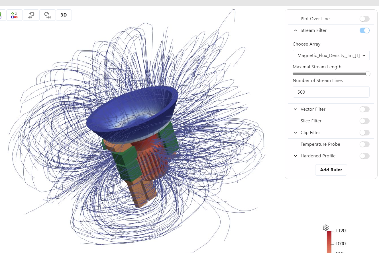
Field plots help explain why a mismatch exists. If the field concentrates in the wrong place, the hardened zone will be wrong later. The field is not the final product, but it is often the fastest clue.

Magnetic field behavior from the shaft scanning case.

Magnetic field stream lines in the CENOS Results Viewer.

What to check in field plots

where the field is strongest
whether the field follows the expected heating zone
whether edges, splines, or corners pull the field away
whether the field pattern changes unexpectedly during motion
whether field concentration matches the hardened area

Field plots are useful when the final result looks wrong but the setup seems correct.

4. Process plots

Power, inductance, current, and voltage plots show whether the electrical side behaves consistently during the scan. These plots are very useful when the final hardening result is off but the geometry looks right.

Performance plots in the Results Viewer. The active power plot is the first default view.

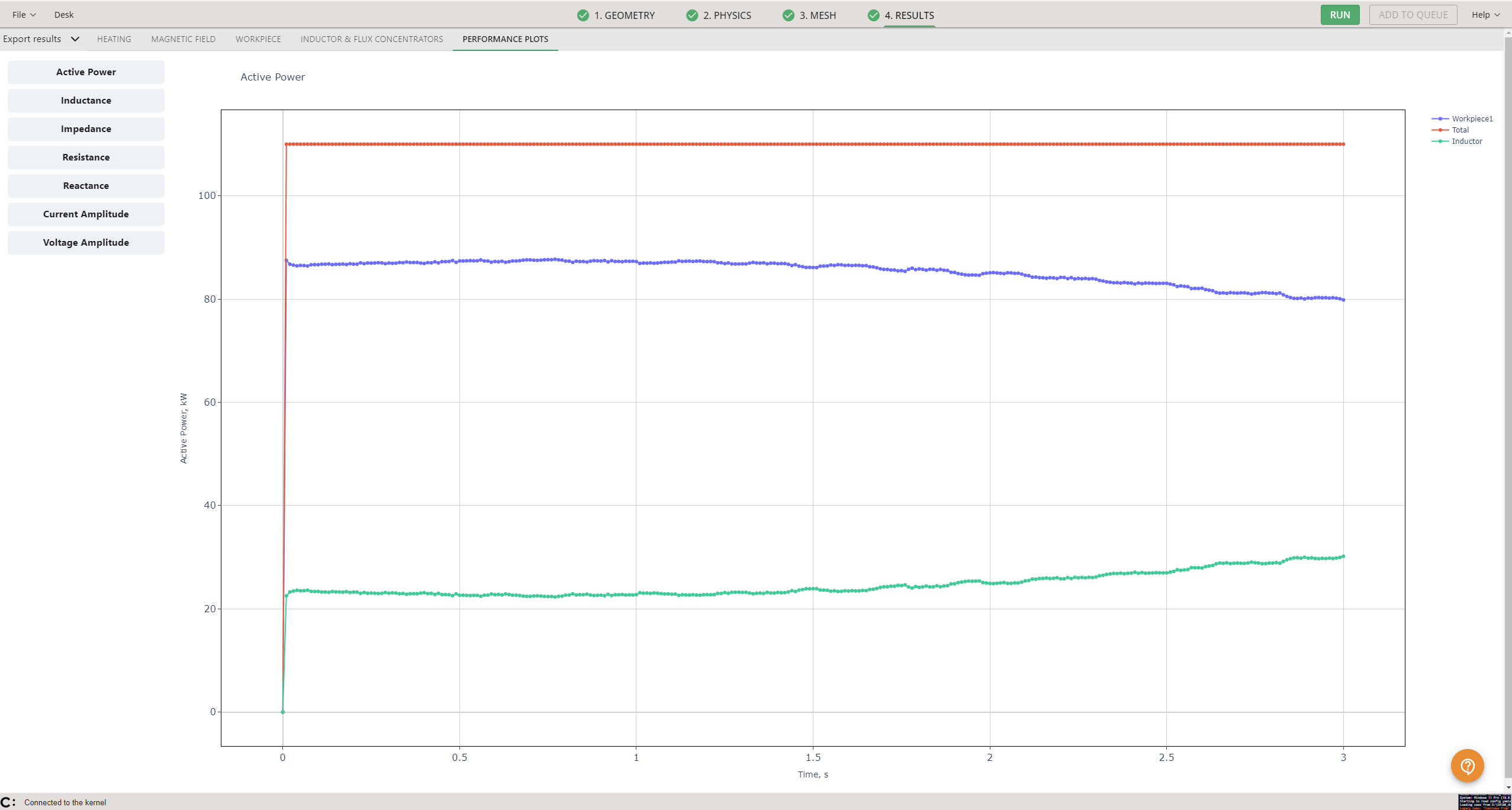
In the shaft case, the documented example reports total power stabilizing around 10.5 kW, with about 5 kW in the workpiece and about 5.5 kW in the inductor. The same case also reports inductance changes during the process, current amplitude stabilizing near 8 kA for Terminal 1, and voltage amplitude settling after the first second. These are not side notes. They help explain whether the process is stable or drifting.

What to check in process plots

does power stabilize when expected
does current follow the expected level
does voltage settle as expected
does inductance change smoothly during the scan
is there any sudden jump that may point to setup or time-step issues
do the plots support the same story as temperature and hardening results

If the plots look unstable, check the setup before trusting the final hardening result.

Why time-step settings can distort interpretation

Time step is one of the most common reasons a simulation looks clean but compares badly with the lab.

The CENOS time-step documentation shows two problems. In static heating, a rough time step can create unrealistic temperature jumps. In scanning cases, the problem gets worse because the inductor moves from one position to another in discrete steps. If the step is too large, the motion becomes jumpy and the thermal pattern becomes unphysical.

Static heating example: rougher time steps distort the temperature history.

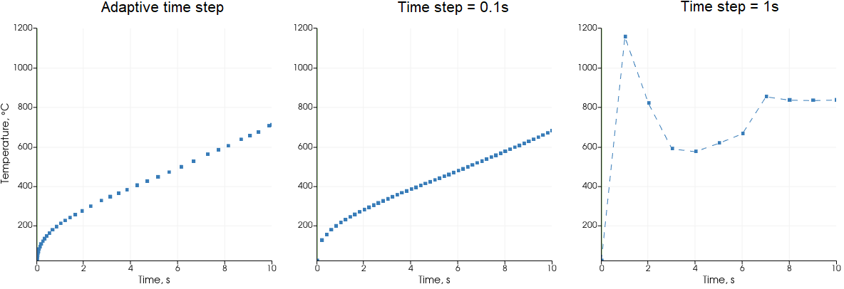
Scanning example: a rough time step makes the inductor jump instead of move smoothly.

So if the lab result and simulation result disagree, check motion resolution early. It is often one of the first things to review.

Time-step review checklist

is the time step small enough for smooth motion
does the inductor move in realistic increments
does the temperature field change smoothly
do the power and current plots look physically reasonable
are you using the same time resolution for comparison points

A poor time step can create a false mismatch or hide a real one.

How to compare with lab data step by step

Start with one fixed reference case. Use one clearly defined geometry, one inductor, one motion path, one cooling setup, and one electrical input.
Make sure the test conditions match. Use the same heating time, scan distance, part position, and cooling delay.
Compare temperature first. Check temperature over time or temperature distribution at known points on the part.
Compare the hardened zone next. Use the same section planes and the same measurement points in both simulation and lab.
If something does not match, then look at the field view and process plots. They often show whether the problem comes from coil coupling, motion, or cooling position.
Change only one thing at a time. If you change power, motion, cooling, and material together, you will not know what caused the difference.

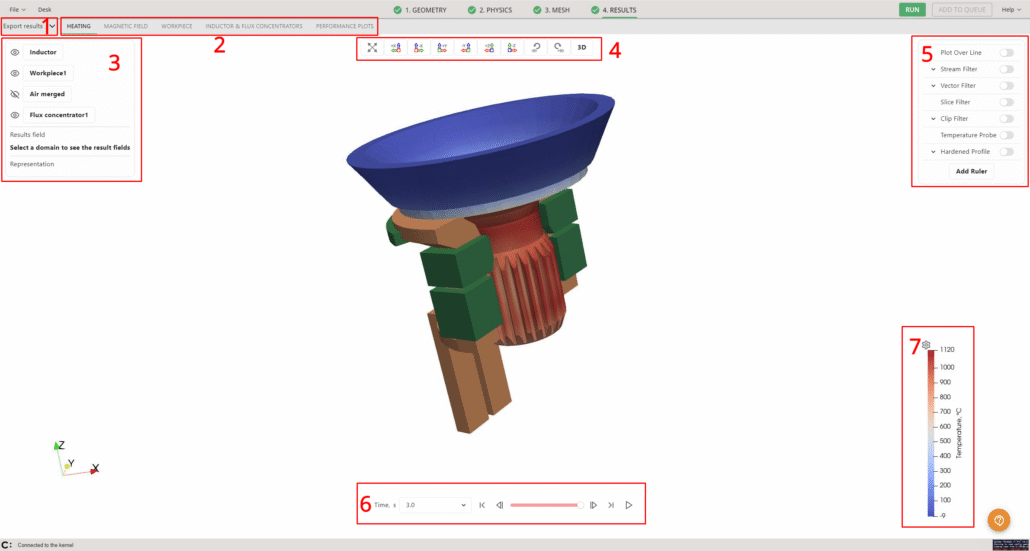
The CENOS Results Viewer helps you check geometry visibility, filters, time steps, and result scales in one place.

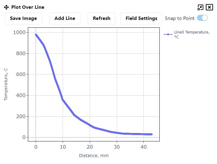
Plot Over Line is useful for comparing gradients across a selected section.

That is the practical reason these viewer tools matter. Validation is not one screenshot versus one lab photo. It is a controlled comparison across several linked outputs.

Practical step-by-step validation checklist

Freeze one reference case.
Confirm geometry, coil, motion, cooling, and electrical input.
Confirm time-step quality for scanning motion.
Compare temperature at fixed positions.
Compare hardened zone at fixed sections.
Check magnetic field if the heated zone is in the wrong place.
Check process plots if the process looks unstable.
Change one input at a time.
Repeat the same comparison points after each change.
Stop when the mismatch is explained by a small and physically reasonable correction.

This is usually a better approach than jumping straight from one final image to one lab cross-section.

What to adjust after the first mismatch

If the mismatch appears in the wrong place, check motion and cooling position first.

If the mismatch has the right shape but the wrong depth, check power, frequency, or the material and hardening assumptions.

If the mismatch changes during the scan, inspect time step and process plots.

If the mismatch is local near edges or splines, inspect the field distribution and geometry details.

The goal is not to massage the model until it flatters the lab. The goal is to find the smallest correction that explains the mismatch and still makes physical sense.

First-mismatch checklist

wrong position -> check motion path, scan speed, and quench location
wrong depth -> check power, frequency, material data, and hardening assumptions
unstable result over time -> check time step and process plots
local edge mismatch -> check geometry detail and field concentration
general mismatch everywhere -> go back to setup basics before changing advanced parameters

This helps keep the debugging process structured.

What good enough correlation looks like in production

Good validation does not mean every pixel matches. It means the simulation predicts the location, shape, and depth trend of the hardened zone closely enough to guide coil and process decisions before you cut metal.

The SMS Elotherm case is the clearest production proof point here. Their team used simulation to test inductor options, met the hardening zone requirements on the first try, then built and tested the selected inductor. The physical test matched the hardening zone predicted by the 3D model.

SMS Elotherm reported that the physical hardening zone matched the predicted zone from the 3D model.

The SMS Elotherm case is the clearest production proof point here.

That is what engineers should aim for. Not a perfect digital twin on a poster. A model that helps choose the right inductor and process settings before the lab campaign gets expensive.

Bottom line

If you want a validation method that holds up, do not start with the final hardening image. Start with the inputs and the process outputs that create it.

For a shaft scanning case, compare geometry, motion, cooling, temperature, hardened zone, magnetic field, and performance plots in that order. Keep the time step under control. Then, if the first comparison misses, adjust one thing at a time until the model and the lab tell the same story.

That is how simulation becomes useful in production. Not because it looks impressive on screen, but because it helps you make the next design decision with less guessing.