
CENOS Mechanics: Deformation, Stress & Microstructure
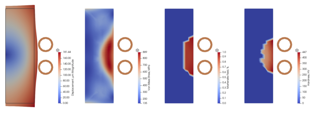
CENOS is capable of calculating different mechanical properties of parts as a result of induction heating and hardening, such as residual stresses, deformation, hardened zone, microstructure and resulting hardness.
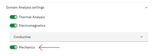
Mechanical calculation can be applied only to domains with Thermal analysis enabled. To enable Mechanics, click on the toggle under Domain Analysis settings for the domain you want to analyze mechanical aspects:
Thermal Stress and Deformation
Induction heating can create steep temperature gradients within a workpiece. The resulting thermal expansion may cause distortion and stress — and, when the material’s temperature-dependent yield strength is exceeded, irreversible plastic strain. The new Mechanics module carries the calculated CENOS temperature field into a mechanical analysis automatically.
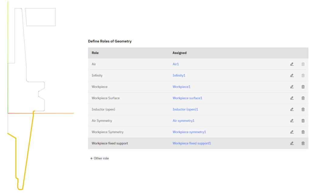
Mechanical supports
Before you attempt to analyze deformation and stress fields of your part, you must define appropriate mechanically fixed faces that won’t be able to deform. Think of a table on which a part is placed before heating, or clamps that fix a part from specific directions, in which part cannot deform.
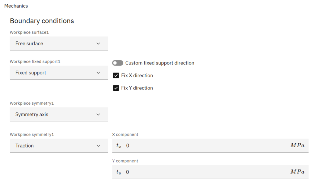
There are 4 types of mechanical boundary conditions available:
- Free surface – this surface can deform freely
- Fixed support – this surface cannot deform in a specific, fixed way
- Fix X, Y, Z directions
- Custom fixed direction: input a vector that specifies the clamp direction
- Symmetry – used for 2D axially symmetrical cases to define mechanical symmetry axis
- Traction – contact surface between 2 objects
Thermoelastic/plastic material properties
Material thermal deformation is described through mechanical material properties and a different plasticity models. Purely thermoelastic deformation requires only 3 material definitions and is enabled by default:
- Young’s modulus (temp. dependent), \( E \)
- Poisson’s ratio, \( \nu \)
- Thermal expansion coefficient (temp. dependent), \( \alpha \)
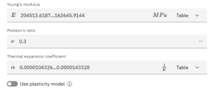
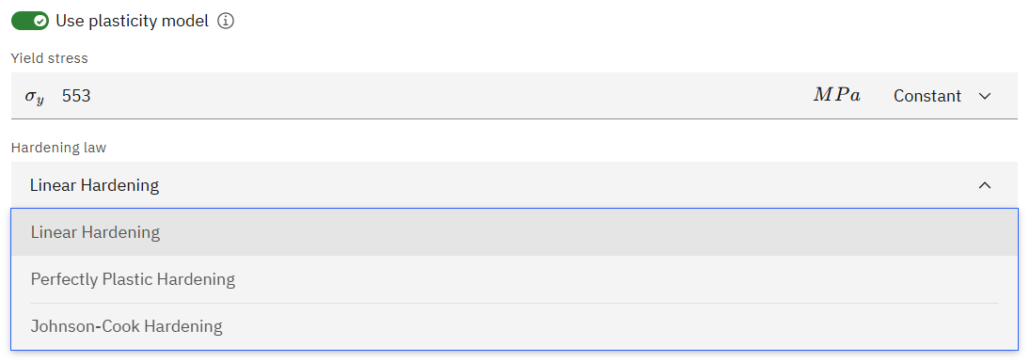
If your applications goes beyond elastic deformations into plastic deformation space, you need to enable “Use plasticity model” toggle to calculate plasticity, irreversible deformation and residual stresses for the material.
Plasticity models
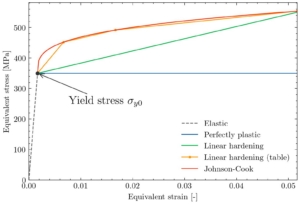
CENOS offers 3 different plasticity models – perfectly plastic, linear hardening and Johnson-Cook hardening.
| MODEL | USE WHEN |
|---|---|
| Elastic | Deformation is expected to remain recoverable, and stress stays below the yield point. Calculated by default when Use plasticity model is disabled. |
| Perfectly plastic | A simplified post-yield model is sufficient |
| Linear hardening | Yield resistance should increase with accumulated plastic strain |
| Johnson–Cook | Temperature-sensitive hardening behavior is required, and the current rate-handling limitation is acceptable |
Here are the 3 hardening models visualized on the stress-strain plot. The Linear hardening law can be modelled as a linear or multi-linear curve.
Perfectly Plastic hardening
Below the yield point, the material behaves elastically, with stress proportional to strain through the temperature-dependent Young’s modulus \( E(T) \). Once the equivalent (von Mises) stress reaches the temperature-dependent yield strength \( \sigma y(T) \), the material deforms at constant stress — the yield surface does not expand with further plastic straining:
\[
\sigma_{\mathrm{eq}} = \sigma_y(T), \qquad \varepsilon_p > 0
\]
This is the simplest post-yield model: it requires only a yield-stress curve, not a separate hardening curve, and it provides a conservative lower-bound estimate of the material’s post-yield strength. Because it assumes zero resistance to further flow once yielding starts, it tends to overestimate plastic strain and residual deformation compared with a hardening material — treat it as a worst-case screening result rather than a precise prediction.
Linear hardening
Beyond yield, the equivalent stress increases linearly with accumulated equivalent plastic strain via a constant hardening modulus \( H \):
\[
\sigma_{y,\mathrm{current}}(T) = \sigma_{y0}(T) + H \cdot \varepsilon_{p,\mathrm{eq}}
\]
This is an isotropic hardening model: the yield surface expands uniformly in all stress directions as plastic strain accumulates, but does not shift (kinematic effects such as the Bauschinger effect on load reversal are not captured). H can also be expressed through an isotropic tangent modulus \( E_t \):
\[
H = \frac{E_t \cdot E}{E – E_t}
\]
Linear hardening is a good first-order choice when you have — or can reasonably estimate — a single post-yield slope but not a full multi-point flow curve, for example, structural and tool steels over a moderate temperature and strain range. Because the hardening slope is held constant, accuracy drops off outside the strain range it was calibrated for, and it does not capture rate effects or strong thermal softening.
Johnson–Cook hardening
The Johnson–Cook model is a semi-empirical flow-stress law that combines strain hardening, strain-rate sensitivity, and thermal softening in one expression:
\[
\sigma_y = \left[\sigma_{y0}(T) + B\,\varepsilon_p^{\,n}\right]\left[1 + C\ln\!\left(\frac{\dot\varepsilon}{\dot\varepsilon_0}\right)\right]\left[1 – T^{*m}\right]
\]
where \(\sigma_{y0}(T)\) is the temperature-dependent yield stress defined in the material’s yield-stress curve, \( B \) is the Johnson–Cook strength coefficient, \( n \) is the hardening exponent, \( C \) is the strain-rate coefficient, \(\dot\varepsilon_0\) is the reference strain rate, \( m \) is the temperature exponent, and:
\[
T^{*} = \frac{T – T_r}{T_m – T_r}
\]
with \(T_r\) the reference temperature and \(T_m\) the melting temperature.
Because it couples yield strength directly to local temperature, Johnson–Cook is the natural choice when thermal softening matters — which is common in induction heating, where the heated zone can be well above room temperature while the surrounding material stays cool.
Best practices & limitations
As with all models, your mechanical analysis is only as good as the definition of the model. Some tips to keep in mind when attempting to set up a mechanical analysis case:
- Constrain only what’s physically fixed, and leave other surfaces free to move;
- Refine the mesh near the coil-heated zone for better deformation and stress resolution;
- Use temperature-dependent properties wherever they matter;
- Start thermoelastic, add plasticity if material yields for simpler first iterations.
CENOS Mechanical module is finetuned for induction heating and hardening simulations, where deformations are relatively small. Because of this, CENOS currently uses a one-way coupling between thermal and mechanical modules, which is accurate while the deformations are relatively small. If the part deforms significantly so that it’s topology changes visibly, resulting calculation might not be as accurate anymore.
Phase change calculation
Simulating the hardening process of steel requires understanding the steel phases formed during heat treatment. This is crucial for predicting material properties and performance.
The CENOS platform includes a Phase calculation model that enables accurate computation of steel phases such as austenite, bainite, pearlite, and martensite.
How to use phase calculation?
Once your geometry is prepared, you can proceed to define the material parameters in the Material customization window. Follow these steps:
- Enable Phase calculation
Check the Phase Calculation option in the Material Customization window. - Define Key Parameters
Specify the following parameters to ensure accurate calculations:- TAc1 (if available): The temperature at which the transformation to austenite begins.
- TAc3: The temperature at which the steel structure becomes fully austenitic.
- TMs: The temperature at which martensite formation begins.
- ts: The start time of the phase change, typically defined as when 1% of transformation occurs.
- te: The end time of the phase change, typically when 99% of the transformation is complete.
- Guidance on TAc1
If the temperature for TAc1 is not available, you may use the value of TAc3 as a substitute.


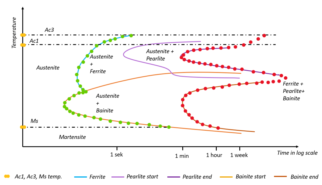
An example of how to get data from a TTT diagram.
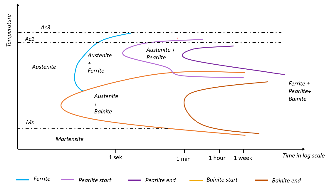
To accurately calculate phase changes, you need data derived from a TTT (Time-Temperature-Transformation) diagram. The TTT diagram provides critical information on the timing and temperature of phase transformations. Below is an explanation of how to interpret and adjust the data:
Interpreting the TTT Diagram
- Combining Phases
- In the Phase Calculation model, bainite, pearlite, and ferrite are treated as a single phase.
- To account for this, connect the start lines for ferrite and bainite (e.g., using green dots in the diagram).
- Similarly, connect the end lines for pearlite and bainite (e.g., using red dots in the diagram).
- Defining ts and te Data
- The start time (ts) and end time (te) for phase changes must be defined within the temperature range from TMs (martensite start temperature) to TAc3 (the temperature at which the structure is fully austenite).
- Extrapolating Missing Data
- If the end line in the TTT diagram does not extend to the TAc3 line (as in the example), you must extrapolate the line. This step is essential to ensure the Phase Calculation Model functions correctly
An example of how to treat TTT diagram to get the data for ts and te:
Hardness calculation
CENOS offers two hardness calculation models designed to estimate steel hardness after heat treatment. Both models will be described in the chapters below.
How to enable hardness calculation models?
- Ensure that thermal analysis is enabled for the domain where you wish to calculate hardness.
- Once thermal physics is activated, Hardness Calculation model and a Phase calculation model will become available.
- Select hardness calculation. Additional input parameters may be required.

Hardness calculation from the table
Key Inputs and Calculation
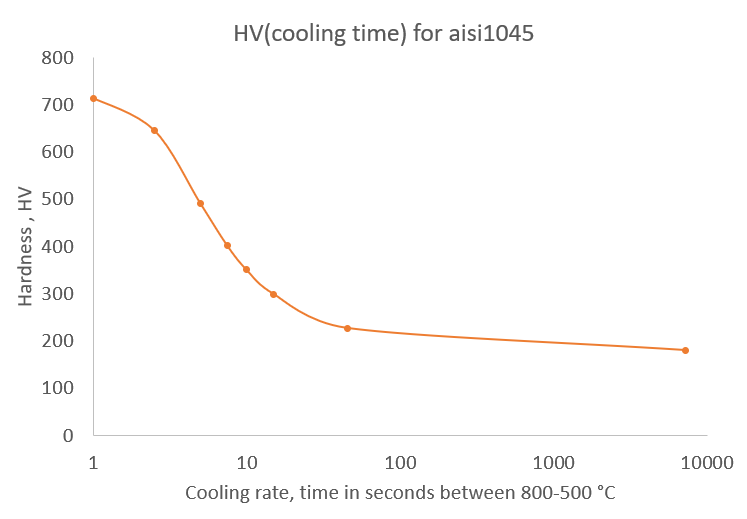
This model calculates material hardness based on cooling time. To use this method, you need to provide data in a tabular format with the following parameters:
- Cooling Time (in seconds)
- Achieved Hardness (in any unit, such as HV, HRC, etc.)
Additionally, you must specify:
- Austenization Temperature (TAc3)
- End Temperature (Tend)
The end temperature (Tend) depends on the data provided in the table. For instance, if the table includes critical cooling times between 800°C and 500°C, set Tend = 500°C.
A reliable source for such material properties is the Ovako Steel Navigator, which provides heat treatment diagrams (see the example below). Similar diagrams to the one needed for this model can be found there.
Another option is to use hardness data commonly found in CCT (Continuous-Cooling Transformation) diagrams. These diagrams display the hardness achieved by the material based on the cooling time elapsed from the austenization temperature (TAc3).
Take note: In the example diagram below, hardness is presented using different scales, such as HV and HRC. Ensure you standardize the scale to avoid inconsistencies in your calculations. [1].
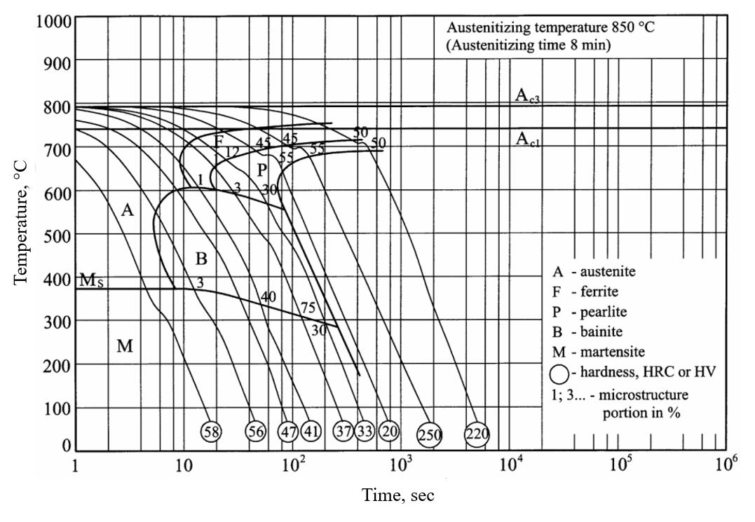
Important: It is important to recalculate the hardness to one scale and use the same units for all data otherwise, the results will be meaningless!
Example
In this case, the end temperature (Tend) is equal to the martensite start temperature (TMs). Since the TMs temperature varies throughout the process, we recommend using the temperature at the beginning of the process—approximately 380°C in this example.
Below is a preview of the model definition in CENOS:

Limitations
The error of calculated hardness depends on the quality of the given HV table data.
References
[1] “Atlas of steels heat treatment”, A. Rose, H. Hougardy, 1972.