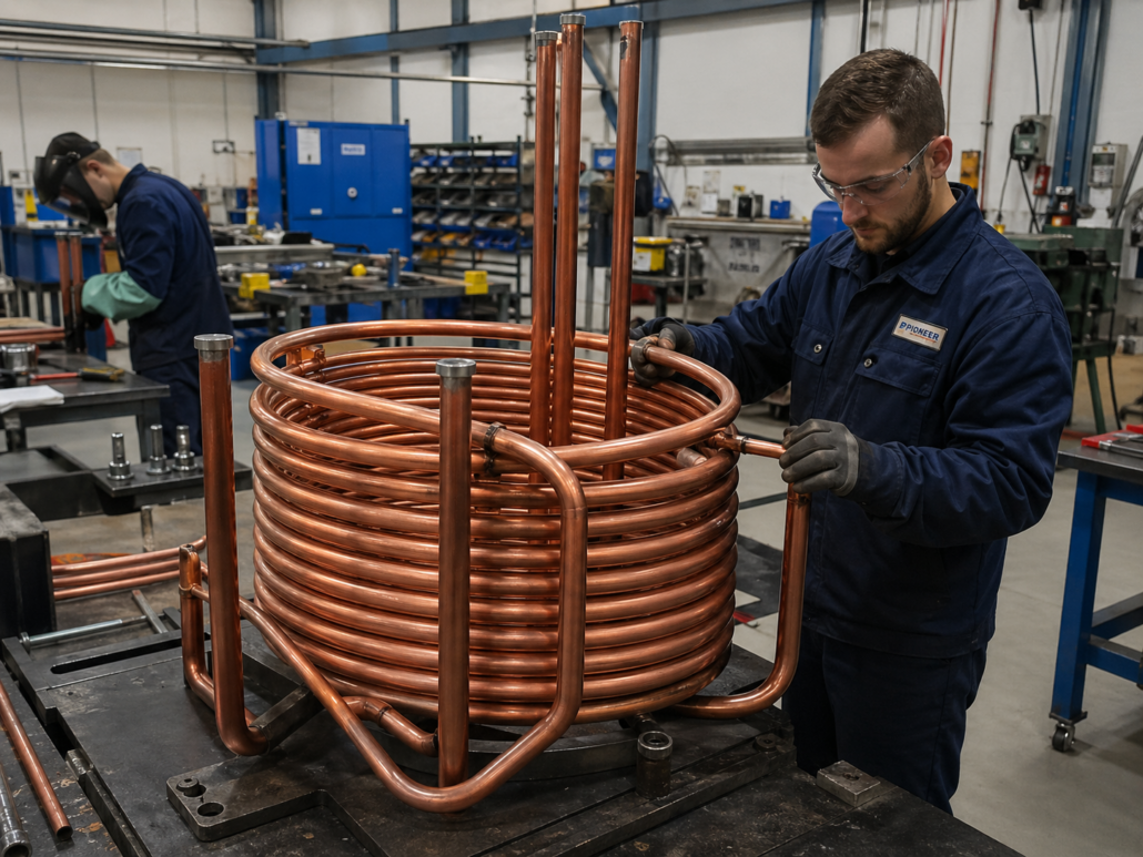
From prototype to production: what breaks first in induction hardening setups
A prototype can prove that a hardening process works.
Production asks a harder question: can the same process run with good output, long coil life, and less time lost to troubleshooting?
That is the real shift from prototype to production. The goal is no longer to get one good result. The goal is to run the line with enough margin.
This article looks at four published examples. Together, they show the same pattern. When a process moves toward production, the first work is usually not about proving the physics. It is about improving cycle time, coil life, setup tolerance, scrap rate, and recovery speed.
What changes from trial to production
A trial usually validates one setup under close attention. Production has to validate output over time.
That difference sounds small on paper, but it changes the engineering target. A prototype run may show that the part can be hardened. Production still has to answer harder questions. Can the line meet the required cycle time? Can the inductor survive long enough to avoid constant changeovers? If the gap shifts or the line needs adjustment, can the team correct the process without stopping for a long series of manual tests?
That is why the article should stay focused on optimization, not on vague process instability. The published cases used here are mainly about improving throughput, extending coil life, reducing scrap, and improving line performance once the process is transferred into production conditions.
Published examples used in this article
The table keeps the comparison compact. It is there to anchor the discussion with numbers, not to slow the reader down.
| Published example used in this article | What started causing trouble first | What the published numbers showed |
|---|---|---|
| CV joint hardening line at GKN Driveline Celaya | Gap sensitivity, and short coil life during line running | Simulation supported a hardening cookbook that cut scrap by 60%, increased coil life from 20,000 to more than 122,000 shots, and improved OEE by 9%. Simulated versus cut-part profile match was reported at 93.8%. |
| Full-float axle scan hardening | Cycle-time push increased sensitivity to position and setup | Optimized scanning improved speed from 9.5 to 11.0 mm/s at 1 kHz and from 6.5 to 9.0 mm/s at 3 kHz. A dual-frequency strategy reached about 11.5 to 11.6 mm/s with lower setup sensitivity. |
| Wheel hub hardening coil | Coil heating and thermal fatigue, even though the part pattern could still be achieved | The original coil failed after about 8,000 to 13,000 parts. The line needed about 50,000 parts per coil. A redesigned coil lasted more than ten times longer than the original. |
| Tool-steel work-roll study | Higher feed rate narrowed the thermal and metallurgical margin | Raising feed rate from 24 to 42 mm/min increased required power from 210 to 370 kW and reduced hardening depth from 50 to 38 mm. |
<h2style=”margin-top: 60px !important;”>Example 1. CV joint hardening: when one good profile is not enough
The GKN Driveline Celaya case is a good starting point because it shows a real production line problem.
The issue was not whether the CV joint could be hardened at all. The bigger issue was whether the process could run with less scrap, longer coil life, and less time lost when the setup moved away from the ideal point.
According to the published CENOS case, simulation was used to build a hardening cookbook for the line. The cookbook focused on how to react when the part-to-inductor gap changed.
The published results were strong:
- scrap reduced by 60%
- coil life increased from 20,000 to more than 122,000 shots
- simulated and measured hardening profile matched at 93.8%
- OEE, meaning overall equipment efficiency, increased by 9%
This is where simulation becomes useful in a very practical way. It is not only about predicting the hardening profile. It is about helping the team react faster when the line drifts from nominal settings.
That is important because production pays for delays twice. First, the line loses output. Second, engineers may need to stop and run manual tests to find the cause. A simulation-backed cookbook helps cut that stop-and-test time.
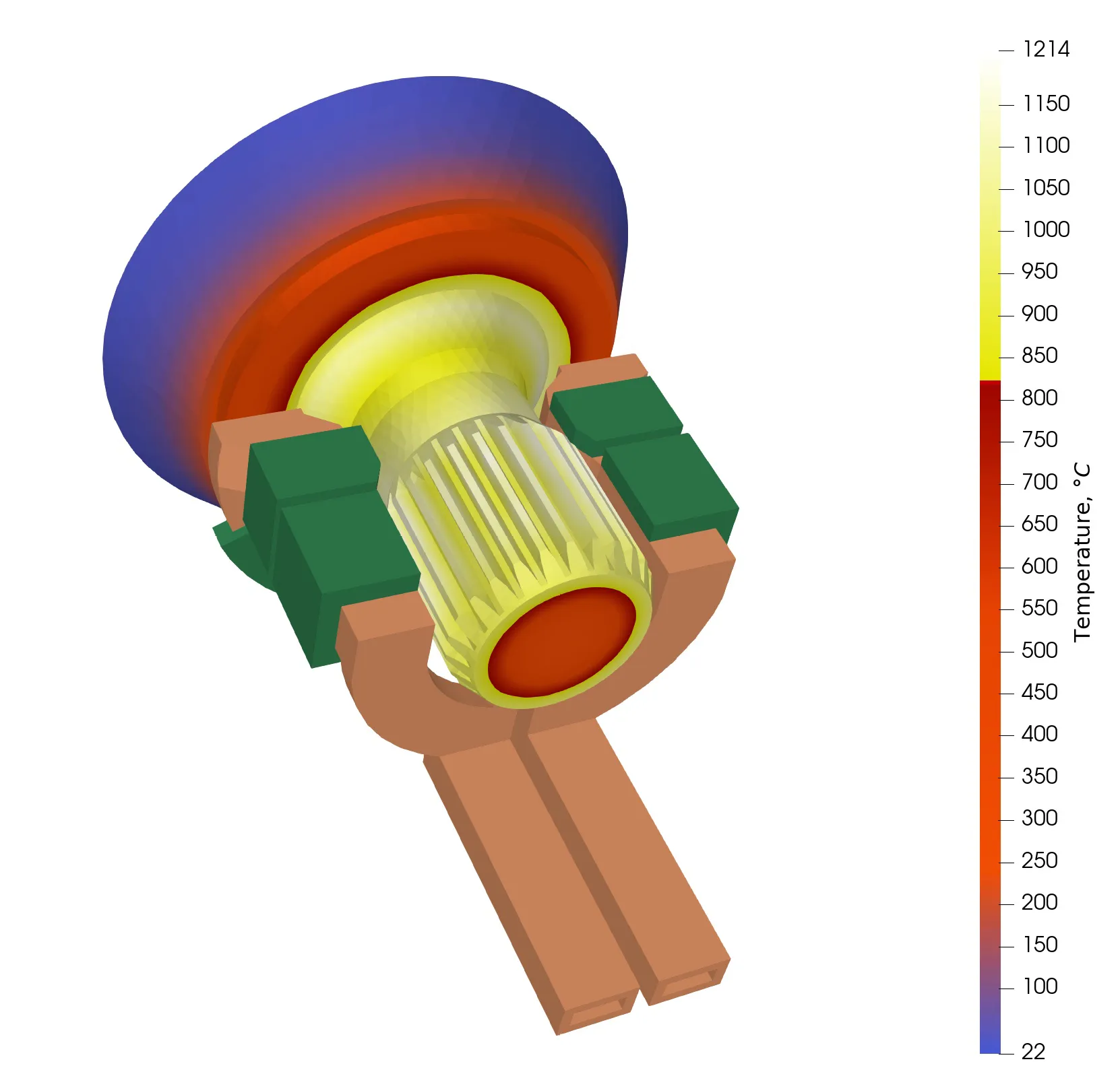
Figure 1. Published CENOS simulation view of the CV joint hardening setup, showing the heated zone around the part. Source: CENOS CV joint case study [2].
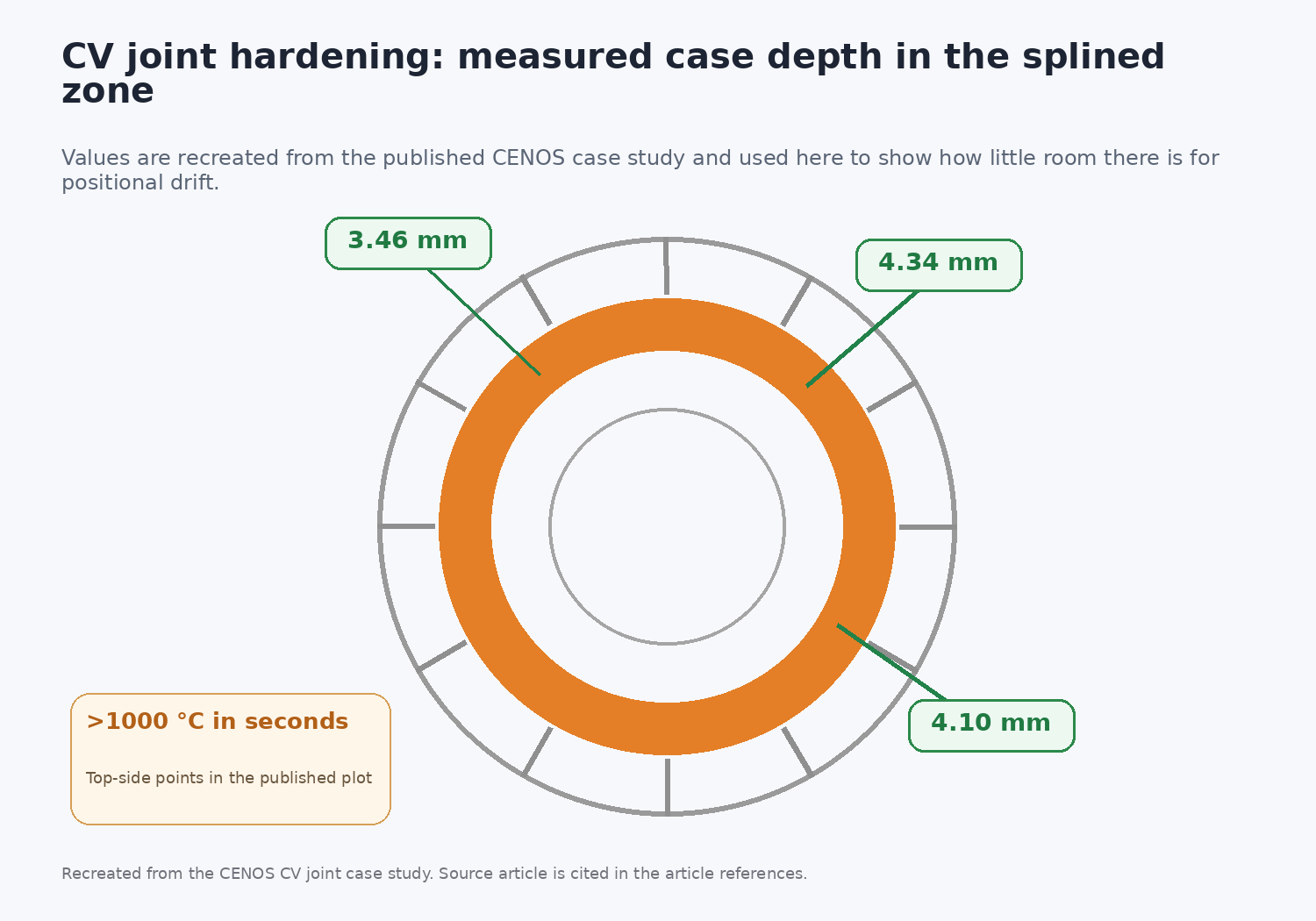
Figure 2. Rebuilt diagram using the case-depth values published in the CENOS article. The point is not the picture itself. The point is how little room there is for the pattern to move. Source: rebuilt from the values published in the CENOS CV joint case study [2].
That makes this case more interesting than a standard validation story.
It is not about getting one good result under ideal conditions. It is about keeping the process under control when the line starts drifting away from nominal. That is often the first real production problem. Not the basic physics of heating, but the repeatability of the heating pattern under normal day-to-day variation.
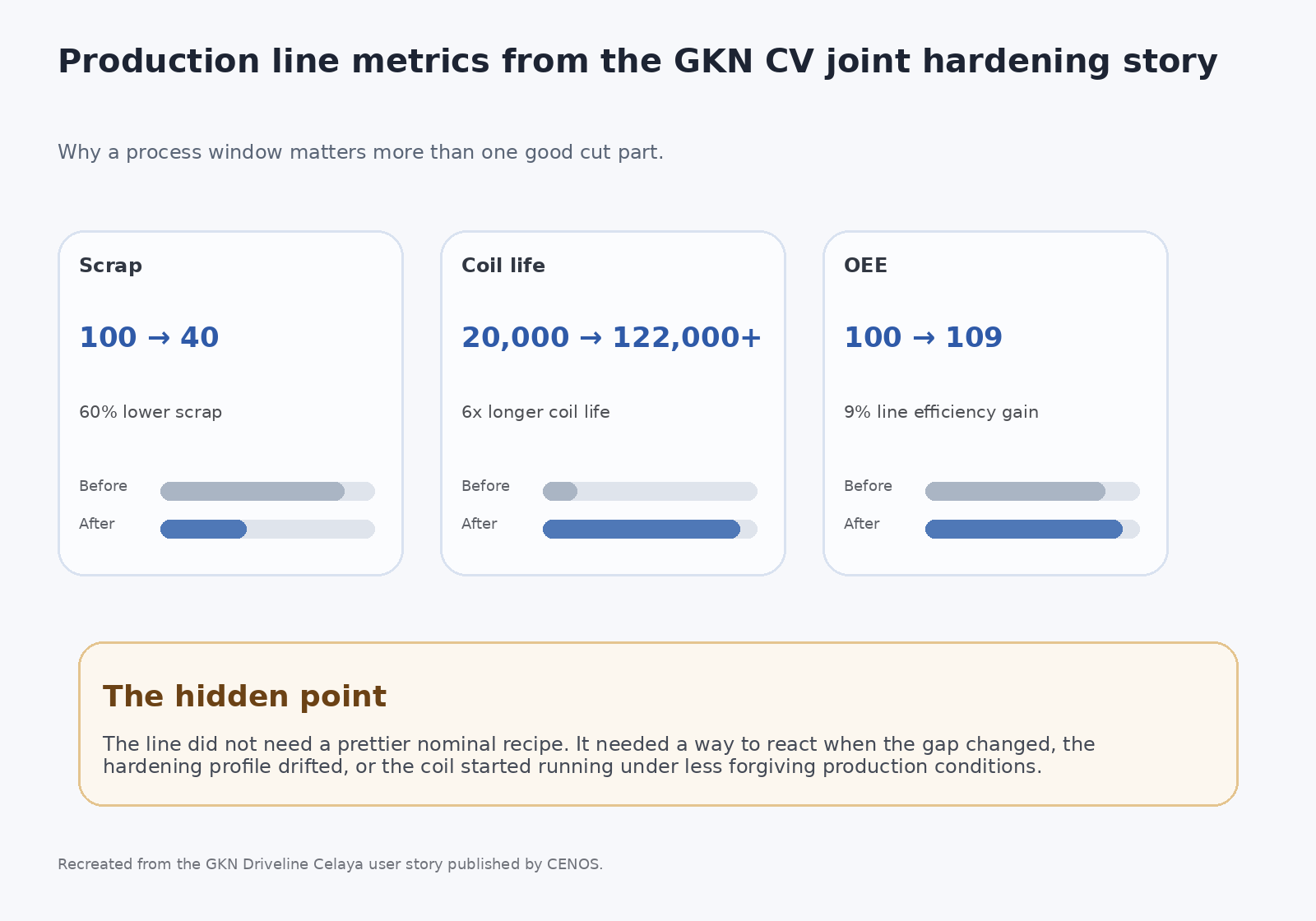
Figure 3. Rebuilt production summary from the GKN CV joint hardening story. Source: rebuilt from the published values in the CENOS GKN user story [1].
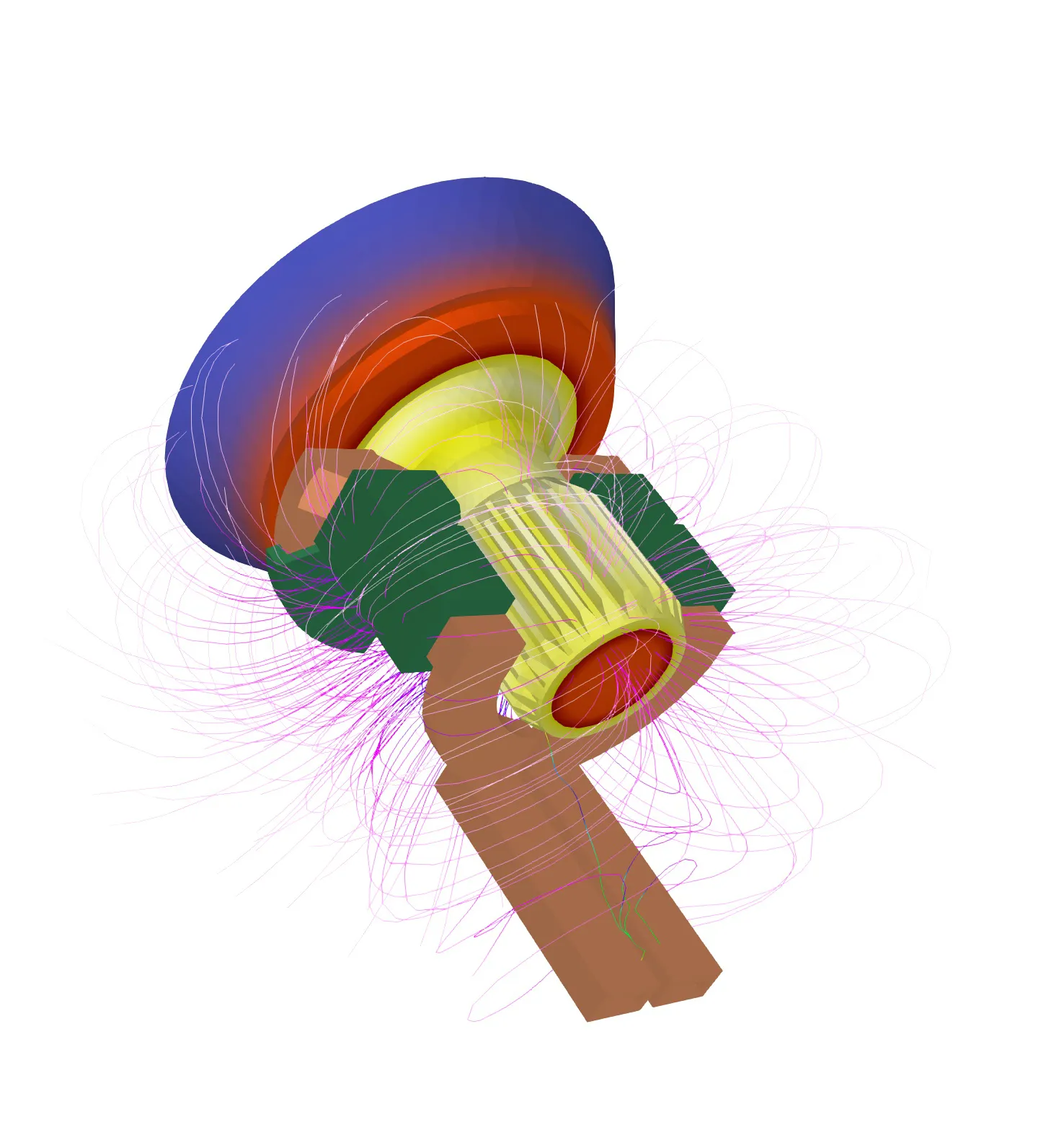
Figure 4. Field-focused view from the published CENOS case, showing why concentrators and local geometry matter around the splined zone. Source: CENOS CV joint case study [2].
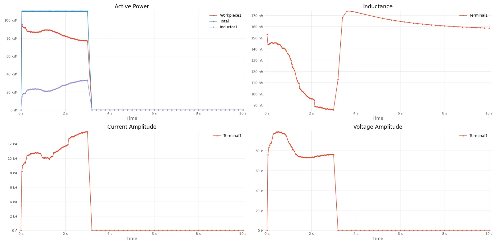
Figure 5. Published process plots from the CV joint case, where active power, inductance, current amplitude, and voltage amplitude are tracked through the cycle. Source: CENOS CV joint case study [2].
What broke first here?
Not the ability to harden a CV joint. The first weak point was repeatability of the hardening pattern when gap, coil condition, and line adjustments stopped staying near the ideal case.
Example 2. Wheel hub hardening: the part pattern survives, the coil does not
The second example comes from an automotive wheel hub hardening study published by Fluxtrol. In this case, the hardening pattern on the part could be achieved. The bigger problem was coil life.
The original single-shot rotating setup failed after about 8,000 to 13,000 parts. The process needed closer to 50,000 parts per coil to run production without constant changeovers.
Failure analysis pointed to copper cracking under the laminations, most likely caused by thermal cycling. The redesign focused on reducing local power density in the coil while keeping the required hardening pattern. The published result showed that the redesigned coil lasted more than ten times longer than the original.
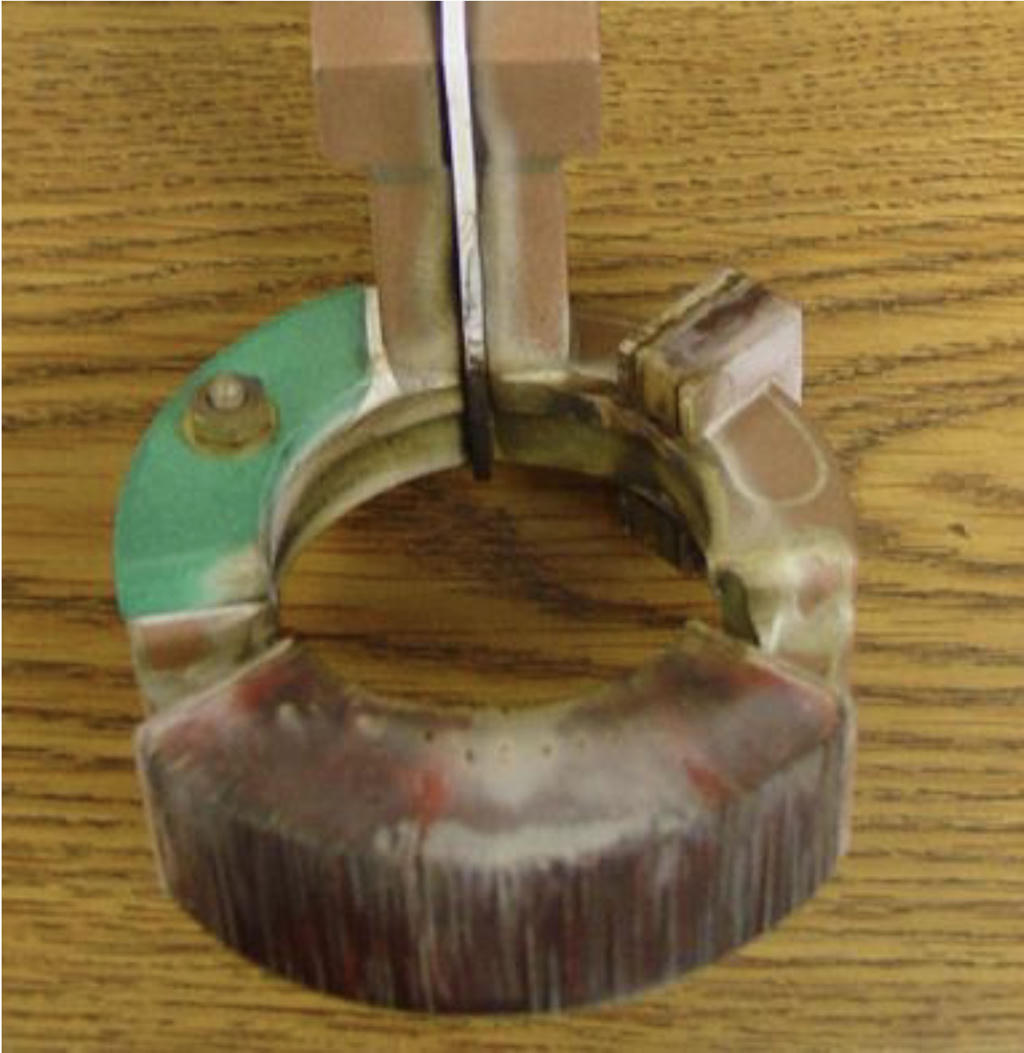
Figure 6. The original production coil after use. Source: Fluxtrol wheel hub case story [3]. |
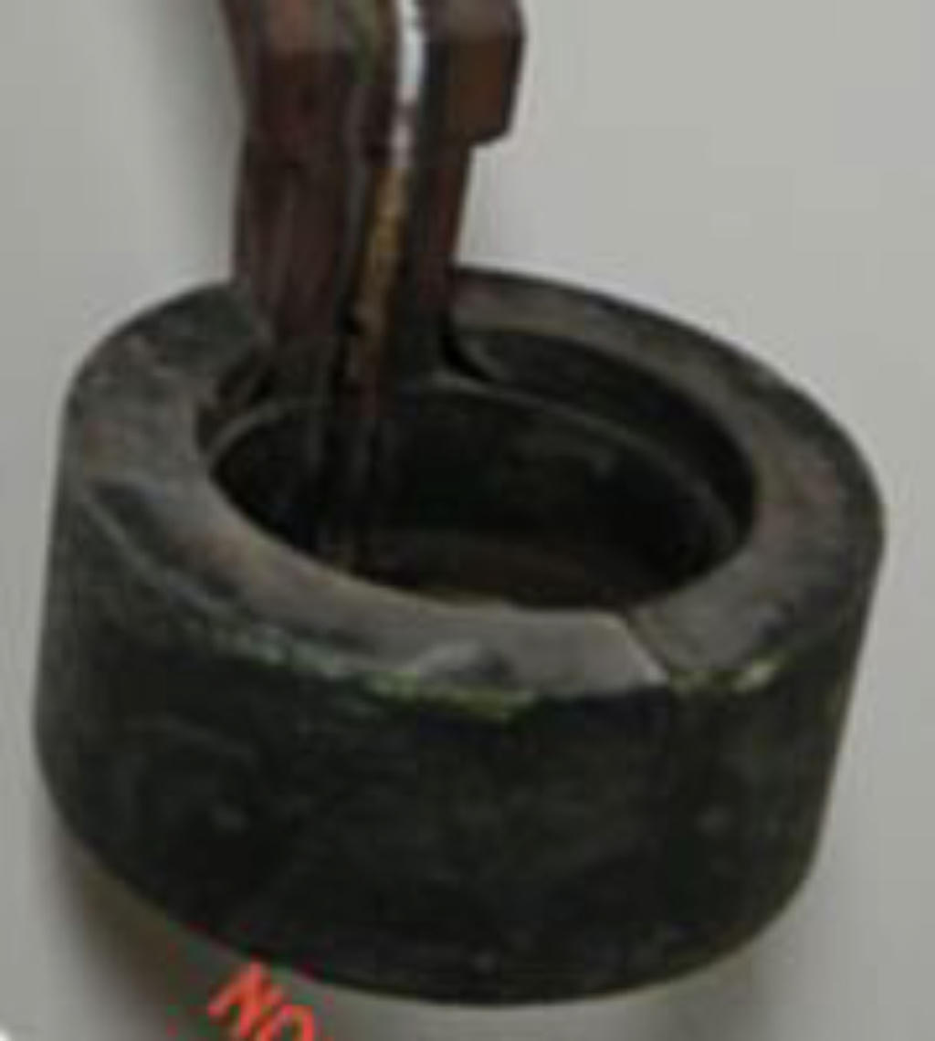
Figure 7. The redesigned production coil after use. Same hardening job, very different life. Source: Fluxtrol wheel hub case story [3]. |
|---|
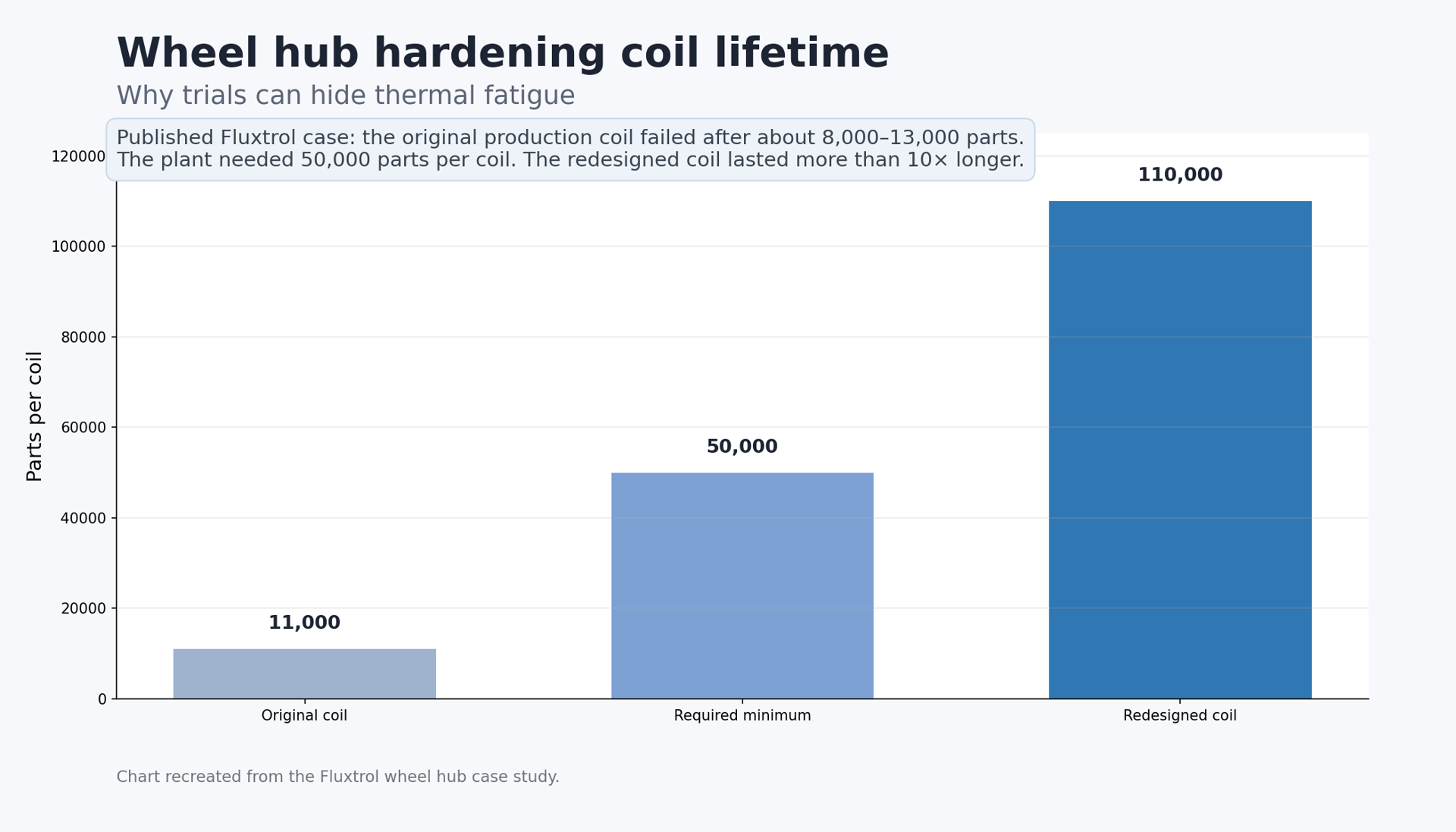
Figure 8. Rebuilt lifetime comparison from the wheel hub case. Source: rebuilt from the published values in the Fluxtrol case story [3].
This example shows an important production risk. Early testing often focuses on the part result and not enough on the tool itself. A few good cut parts can make the setup look ready, even when the coil is building up heat, stress, and damage in the background.
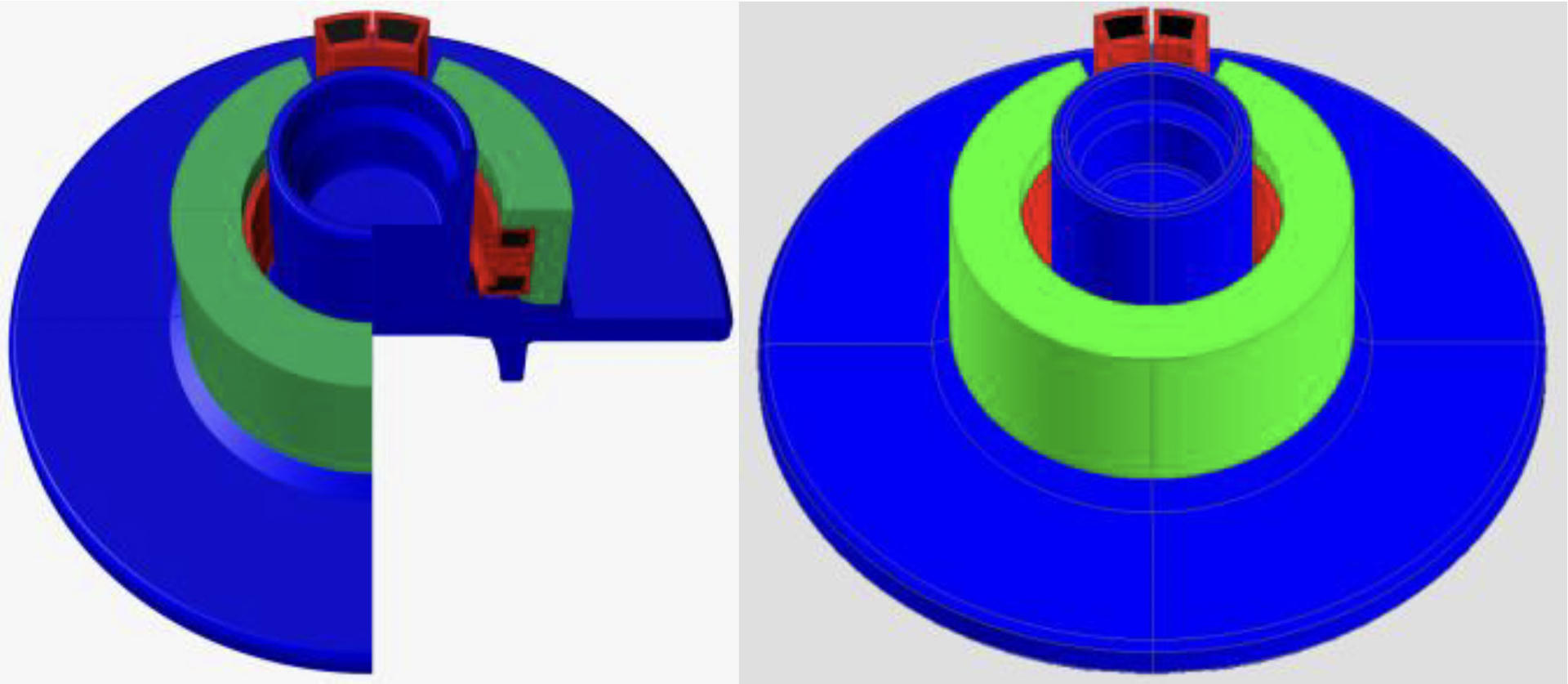
Figure 9. Model view used for the later 3D investigation. Source: Fluxtrol wheel hub case story [3].
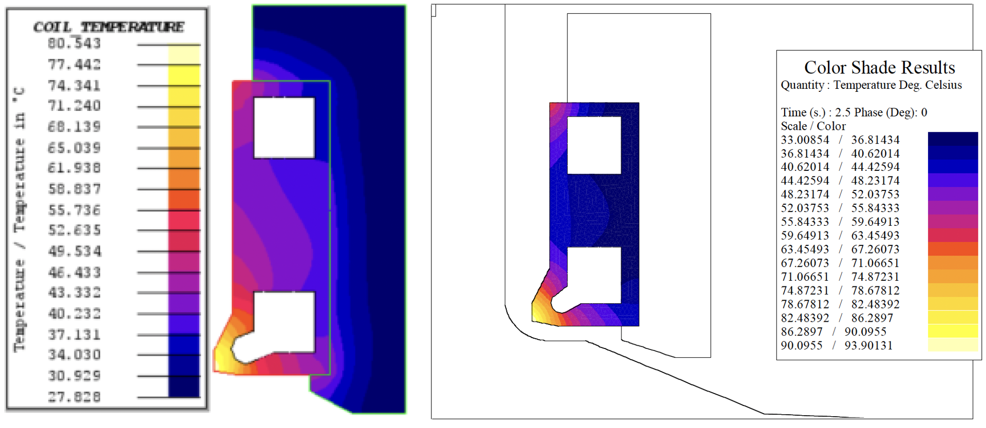
Figure 10. Published thermal comparison of the redesigned coil. Source: Fluxtrol wheel hub case story [3].
That means the next problem is not always part quality. Sometimes it is tool durability under repeated production loading.
If a team validates only the part response and ignores coil thermal behaviour, the line will eventually expose the weakness. Usually in the most expensive way possible.
What broke first here?
Not the part pattern. The first weak point was coil thermal durability under repeated production cycling.
Example 3. Axle scan hardening: a faster setup also becomes a touchier setup
The third example is a full-float axle scan-hardening study, and it is useful because it shows how cycle time and positioning tolerance start arguing with each other the moment the process is pushed harder. The paper describes how standard two-turn coils can provide high speed, but make fillet hardening difficult without overheating the adjacent stem. To solve that, the coil may be placed very close to the axle fillet, around a 1.5 mm gap. That helps, but it also makes accurate coil position and the power-time-speed recipe much more critical.
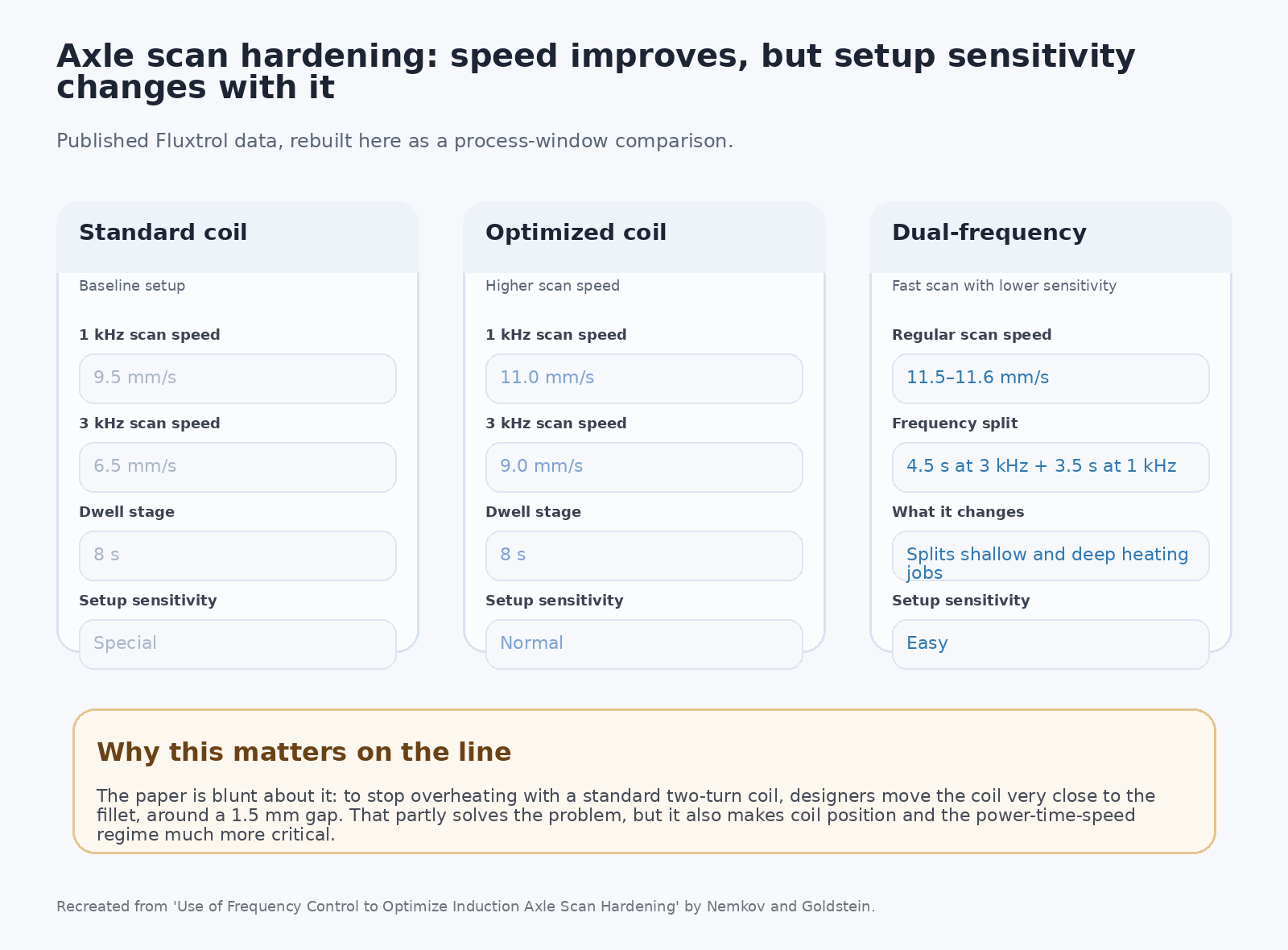
Figure 11. Rebuilt comparison of the published axle results. Source: rebuilt from the published Fluxtrol axle paper [4].
The published values are worth keeping together because they tell a full story. At 1 kHz, scan speed improved from 9.5 to 11.0 mm/s when the optimized inductor was used. At 3 kHz, speed improved from 6.5 to 9.0 mm/s. Then a dual-frequency strategy used 4.5 seconds at 3 kHz followed by 3.5 seconds at 1 kHz and ran around 11.5 to 11.6 mm/s, while also reducing process sensitivity relative to the more touchy setup.[4]
That makes this example especially relevant now. CENOS has implemented dual-frequency functionality, so this is a strong candidate for a dedicated follow-up use case. Replicating a similar study in CENOS would show not just that dual frequency exists, but how it changes the trade-off between speed, profile control, and production robustness.
This example points to the third thing that often breaks first in production transfer: process sensitivity once cycle time is tightened. In trials, a careful setup and generous dwell can look perfectly fine. Production usually asks whether the same outcome still holds when speed increases and the setup has to be less precious.
What broke first here?
The first weak point was process tolerance to position and timing. The geometry still could be hardened, but the operating window became tight enough that the line had to treat setup accuracy like a hard process parameter.
One more case: part variation can expose a narrow window very quickly
The fourth source is a 2024 SpringerOpen paper on induction hardening of tool-steel work rolls. It is useful here because it shows how sharply metallurgical outcome can shift when line speed changes. In that study, increasing feed rate from 24 to 42 mm/min pushed required power from 210 to 370 kW, while hardening depth dropped from 50 to 38 mm.[7] That is a big move in both energy demand and final result, and it happened without changing the frequency target concept.
This matters because production scale-up rarely changes just one knob. Once throughput pressure enters the room, the system becomes less forgiving. Then the ordinary spread in part condition and geometry starts biting harder. A recipe that looks fine in the centre of the process window can become unstable near the edges very quickly.
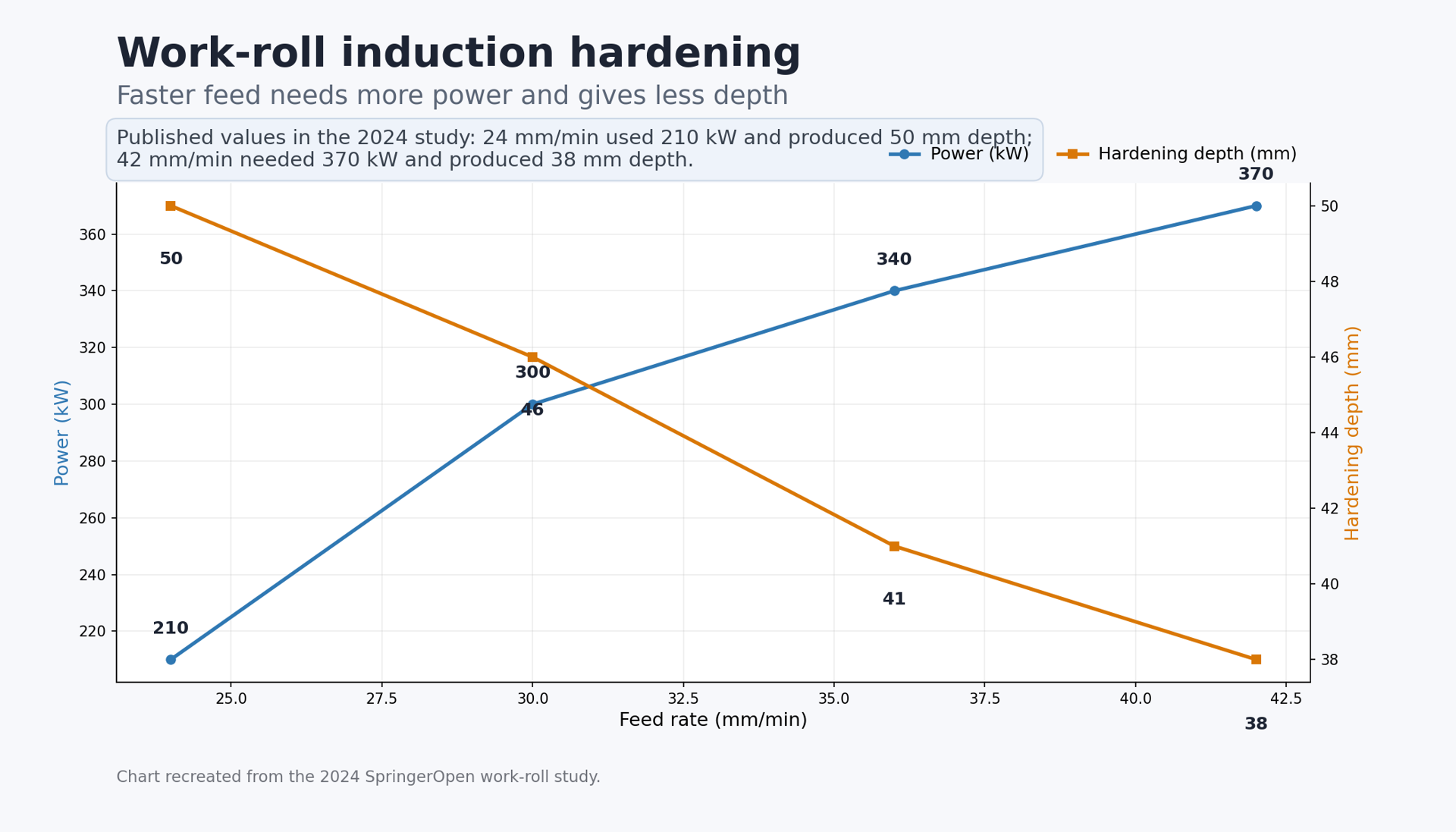
Figure 12. Rebuilt chart from the work-roll study, showing the trade between feed rate, power demand, and hardening depth. Source: rebuilt from the published values in the 2024 SpringerOpen paper [7].
So what should teams check earlier?
The practical move is not to validate one nominal recipe and declare victory. It is to stress the process around that recipe on purpose. The earlier teams do that, the earlier they find out what breaks first.
- Hot coil vs cold coil
Check whether copper temperature or nearby metal shifts the pattern from one cycle to the next. - Gap and position offsets
Move the part or coil inside the tolerance band on purpose and watch which zone moves first. - Faster scan
Test the production push early, before the line asks for it after the design is already frozen. - Part-to-part spread
Try the process on the edges of the likely production distribution, not only on tidy nominal parts. - Tool-life risk
Watch coil temperatures and local hot regions, not only the cut part and the target case depth.
The relevant question is not simply whether simulation can replace a prototype loop. The more useful question is whether it helps engineers map how motion, cooling, quenching, gap, temperature-dependent material behaviour, hardness profile, and electrical results such as power or current change when the process stops being ideal. That is the kind of information that helps during production transfer, not just during a demo run.
Finally, if something breaks in production process, they have to stop production until they figure out what is causing the issue. Or they have to stop the production to carry out manual tests. Simulations help avoid this and run production 24/7.
Conclusion
When induction hardening moves from prototype to production, the first thing that usually fails is not the process itself. It is the belief that the process has enough margin.
The examples in this article all show the same pattern. In the CV joint case, small position changes turn into scrap and line losses. In the wheel hub case, the part pattern still works, but the coil slowly wears itself toward failure. In the axle case, higher throughput makes position and timing much more sensitive. The work-roll data shows the same thing from another angle: when speed changes, the thermal and metallurgical response changes with it.
That leads to a better engineering question.
Not only, “Does the prototype work?”
But, “What breaks first when we run this like production?”
That is where the useful work begins. It is the point where a team stops celebrating one good trial result and starts building a process that can hold up on the line.
References
- CENOS, “GKN Driveline Celaya increased overall equipment efficiency (OEE) for a CV joint hardening line by 9%.”
- CENOS, “Single-shot hardening of CV (constant velocity) joint: case study.”
- Fluxtrol, “3D Simulation of an Automotive Wheel Hub and Induction Hardening Coil to Solve Coil Lifetime Issues.”
- Valentin Nemkov and Robert Goldstein, “Use of Frequency Control to Optimize Induction Axle Scan Hardening,” Fluxtrol PDF.
- CENOS, “Resources” page with related induction-heating case studies.
- CENOS, “Induction Heating” documentation, including motion, cooling, quenching, input types, and result analysis.
- A. Šapek et al., “Effect of feed rate during induction hardening on the hardening depth, microstructure, and wear properties of tool-grade steel work roll,” Journal of Materials Science: Materials in Engineering, 2024.
Live sources used for this draft: [1] [2] [3] [4] [5] [6] [7]
