Optimizing solidification simulation in electromagnetic stirring applications: case study
In the field of advanced manufacturing, achieving precision in solidification processes, particularly under the influence of electromagnetic stirring (EMS), brings several challenges to the table. In this case study we want to look into a detailed simulation workflow focusing on overcoming bottlenecks in transient simulations by using steady-state solutions as initial conditions. By applying these techniques, engineers can significantly reduce simulation time while maintaining accuracy.
The attached image materials in this case study show us visual insights into the evolving states of the solidification process under different conditions, with each snapshot demonstrating the changes between velocity, temperature gradients, and melt fraction.
What is the challenge?
Solidification in the presence of electromagnetic stirring is transient and requires precise simulation of hydrodynamics and electromagnetics. To achieve accurate results, it demands the following basics to be covered:
Transient complexity: Fully transient simulations for both hydrodynamics and electromagnetics are time-intensive and produce enormous amounts of data.
Steady-state assumptions: Steady-state simulations, while faster, can introduce inaccuracies if results are not carefully interpreted, as the steady state does not inherently reflect physical stability in solidification.
Iteration-dependent comparisons: With solidification evolving over iterations, comparison across simulations becomes unreliable without consistent parameters.
Simulation time: Transient simulations can take weeks, creating inefficiencies for engineers needing rapid results for real-time decision-making.
The challenge is to balance accuracy with computational efficiency to find a method that delivers meaningful insights in a shorter timeframe.
What is the solution?
A hybrid simulation approach was devised, combining steady-state and transient methods to balance speed and accuracy:
Steady-state initialization: Simulations begin with a steady-state solution to establish baseline hydrodynamic conditions in hours rather than days.
Transient refinement: These results serve as the initial condition for transient hydrodynamic simulations, allowing the system to stabilize further.
Selective transient electromagnetics: Transient electromagnetics are activated only when necessary, minimizing the computational load while capturing critical dynamics.
Iteration control: Steady-state simulations were artificially prolonged to advance solidification, enabling consistent comparisons across cases.
This tiered approach reduces the time needed for transient simulations while maintaining accuracy, with the steady-state results providing a practical foundation for further analysis.
Let’s look at the simulation visuals and explain what can we see.
The two images provided illustrate the solidification process in a crucible influenced by electromagnetic stirring (EMS). Below is a detailed analysis based on the key parameters visualized.
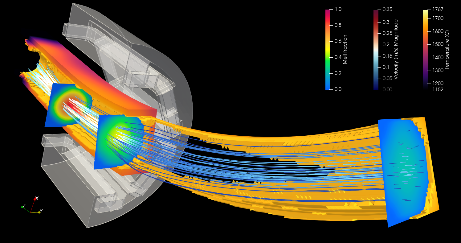
Steady-state simulation with stirrer coil voltage 2V
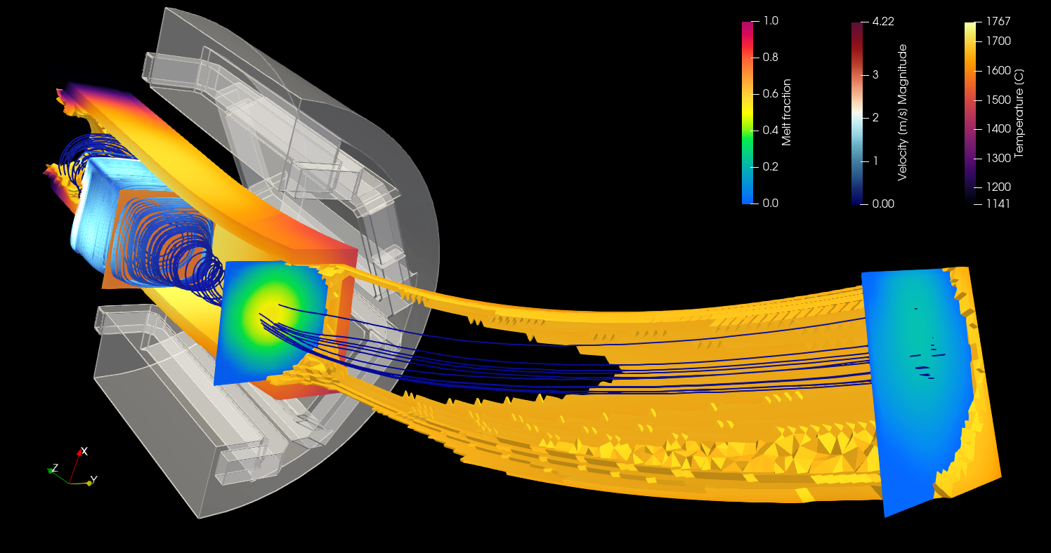
From steady-state results, it looks like more intensive stirring leads to better solidification. However, simulation with 2V finished at iteration 8481, but simulation with 10V was continued from the previous calculation with few restarts and the final result is displayed at iteration 21165.
Melt fraction
- The melt fraction ranges from 0 (fully solid) to 1 (fully liquid).
- In the first image, the melt fraction near the electromagnetic stirring area is close to 1, indicating a mostly liquid state.
- In the second image, the melt fraction shows a larger zone transitioning towards solidification, particularly near the edges of the crucible, where the value drops below 0.2.
- The melt fraction gradient reflects the efficiency of EMS in keeping the material near the stirring region in a liquid state, while peripheral areas begin to solidify as temperature gradients intensify.
Velocity magnitude
- Velocity magnitude ranges from 0 m/s to a maximum of approximately 4.22 m/s in the second image.
- In the first image, velocities are relatively low, with the highest value near 0.35 m/s, indicating limited stirring and flow dynamics.
- In the second image, velocities are significantly higher, especially near the electromagnetic stirring region, where they exceed 3 m/s, showcasing enhanced stirring effects.
- The stronger electromagnetic fields generate a more intensive stirring force, which in turn leads to increased velocity. We can see this in the second image, where mixing is improved. This improves mixing but could also contribute to higher thermal gradients.
Temperature distribution
- Temperature varies from 1152°C to 1767°C.
- In the first image, the temperature is more uniformly distributed, with most of the melt above 1500°C, ensuring a homogeneous liquid state in the central region.
- In the second image, the temperature gradient becomes more pronounced. The areas near the walls are cooler (below 1300°C), while the central stirring region remains above 1600°C.
- The temperature gradient corresponds to the transition from liquid to solid. The enhanced stirring in the second image creates a more localized high-temperature zone in the center while allowing cooler regions to solidify faster.
Overall dynamics
First image: Represents an initial, relatively uniform state with moderate stirring and limited solidification. The process is in the early stages, with melt fraction and temperature uniformity reflecting the dominance of the liquid phase.
Although steady-state solution has converged, we have to keep in mind that we are modelling a transient process. It means that, although each additional iteration gives very small contribution to the solidification front, overall after thousands of iterations, the changes can be quite noticeable.
Second image: The second image shows simulation, which has been continued from the previous calculation results. In this simulation we have increased coil voltage from 2V to 10V, thus strengthening the electromagnetic stirring intensity.
Here we can see that the increased mixing has disrupted the solidification and melted the already sold regions near the coils, where the electromagnetic mixing is the strongest. On the other hand, additional iterations have advanced the growth of the solid region further down the channel, where the electromagnetic mixing is no longer forcing the flow.
The following two simulation videos provide details about the solidification process under different conditions. Both simulations use electromagnetic stirring to influence the melt’s hydrodynamics, but they differ in duration and parameter focus.
First video (duration: 80 seconds): This video shows a harmonic transient simulation. It visualizes how stirring gradually impacts the melt over an extended period. The simulation highlights the interaction between electromagnetic forces and the melt dynamics, showcasing strong, oscillatory stirring patterns. The transitions are smooth and demonstrate how the melt reacts to varying electromagnetic fields.
Second video (duration: 10 seconds): The simulation focuses on transient conditions with fixed temperatures. It captures a more immediate and localized response to electromagnetic forces, emphasizing the interaction in a confined time window. The flow patterns are sharper, and the temperature gradients stabilize faster due to the fixed thermal boundary conditions.
What is the result?
The optimized workflow improves simulation efficiency while preserving the accuracy of results.
Time savings: Steady-state simulations reduced setup time from weeks to a few hours, with transient refinement completing in days instead of weeks.
Consistent results: Using steady-state results as an initialization point ensures that transient simulations converge more quickly and reliably.
Clear visual insights: The attached images illustrate the evolving states of the simulation. For example:
- Early steady-state results show uniform melt distribution.
- Advanced transient stages reveal the detailed velocity field, temperature distribution, and solidification patterns.
Improved decision-making: Engineers can confidently analyze solidification dynamics without waiting for prolonged simulations, enabling faster iteration on design and process optimization.
Conclusion and future direction
In the steady-state simulations, a harmonic time-averaged approach was applied to electromagnetic stirring (EMS) while solving the hydrodynamics in a steady-state framework. This method allowed for faster computation, achieving results within hours instead of the days or weeks required for fully transient simulations.
However, since solidification evolves over iterations in steady-state calculations, comparisons between different cases were only meaningful when performed at similar iteration levels to avoid misleading conclusions.
Additionally, while the steady-state results provide valuable insights into flow structures and temperature distributions, they do not inherently reflect a fully stabilized physical state, as solidification is a transient process by nature. To address this, the steady-state simulations were extended artificially to observe further solidification development.
The implications of this approach are significant: it enables engineers to quickly evaluate flow patterns, temperature gradients, and stirring efficiency before investing in computationally expensive transient simulations.
Moreover, using steady-state results as initial conditions for transient calculations accelerates convergence and enhances simulation accuracy, making it a practical and efficient strategy for optimizing electromagnetic stirring processes.
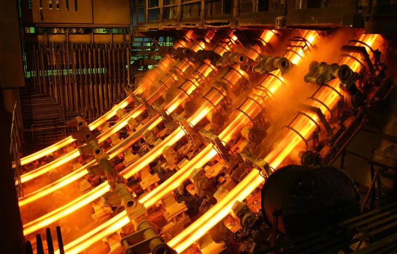
Credit: Illustrative image of continuous casting for this case study post is from “Fine Metal” article.
