IH Results Viewer

This article is a walkthrough of the built-in CENOS IH Results Viewer. Here you can find out about different results manipulations, filters, views and export options.

Overview

CENOS IH Results Viewer is divided into multiple parts. You can see an image below:

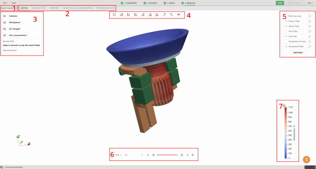
1. Different results export options, for example, current view image, animations.
2. Results tabs with different default filters enabled, for example, HEATING, MAGNETIC FIELD, PERFORMANCE PLOTS.
3. Results and Visibility – here you can choose which geometry objects are shown, how they are shown and what values (Temperature, Current Density, etc.) are shown.
4. Main view positioning options. With these you can center the geometry, see the geometry from a specific plane, turn it 90 degrees and switch between 2D and 3D views.
5. Result filter options.
6. Time selection. Here you can use the dropdown menu to select a specific timestep, use the slider or click the play button to see the heating visually.
7. Result value scale.

Results and Visibility

On the left side menu you can see the geometry object selection. There you can toggle visibility for which objects you see by pressing the eye icon.

When you click on an object, you will see a more detailed menu show up – there you can choose how the object is displayed – what result fields it shows. It can be temperature, current density, just solid color etc.

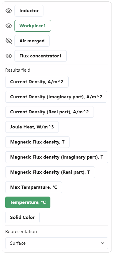
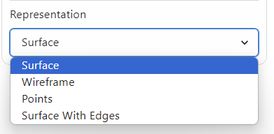
You can also choose whether the object is represented as a full object, a wireframe, as points or a surface with edges.

Once you have chosen the representation, you can see on the right side a scale – you can modify it as well.

If you click on the gear icon, you will see a menu show up. From there you can choose three ways to rescale the values:

1. Rescale to Data Range – meaning to the current timestep you have selected;
2. Rescale to Custom Range – you can select the lowest and highest values to be displayed;
3. Rescale over Time – the scale will show all values that have appeared during the calculation.

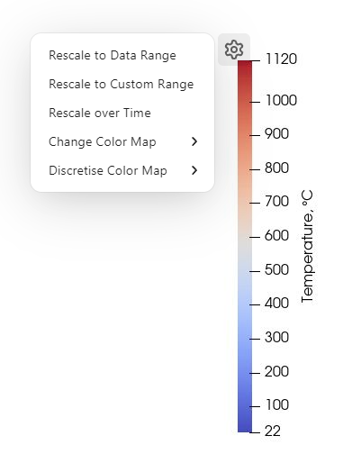
Along with rescaling, you can choose a diferent color map – four preset options, and you can discretize the color map – the higher value you set (1 to 256), the smoother the gradient and visualization of the colors.

Result Filters

On the right side you can see a selection of filters used for deeper result analysis.

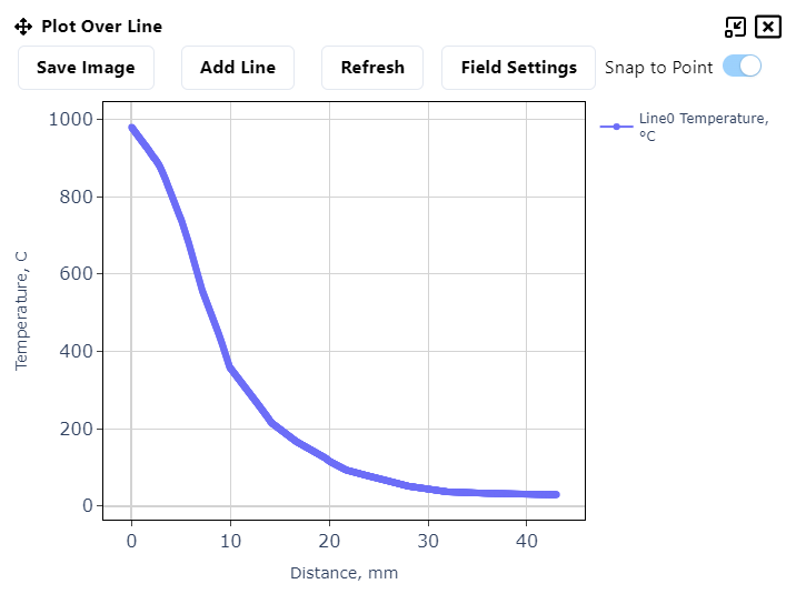
Plot Over Line

This filter allows you to see selected results (temperature, current, etc.) over the drawn line.

When enabling the filter, you will see a new window popup. In this window you can save the created plot image, click ‘Add Line’ when you want to create a new line, you can Refresh the view, change the Field Settings and toggle the snap to point option.

When you add a line, it will appear in the 3D visualization window. You can drag the ends of this line to your desired spots on the geometry. If you have enabled Snap to Point, the ends of the line will snap to the closest mesh element to the place you dragged it to.

Once you have set the line as you wish, click Refresh to see the plot. You can add as many lines as you wish.

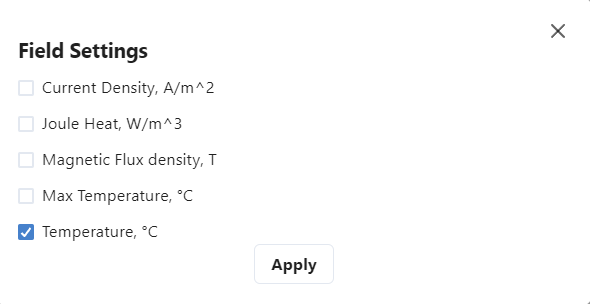
If you want to see some other results, select ‘Field Settings’. A new popup window will open where you can choose other results to display instead.

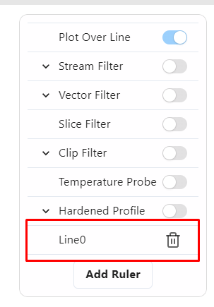
If you decide that you do not want to see the created line, you can click on its name in the Plot Over Line popup window. If you want to delete the line permanently, you can click on the trash icon on the right side – under all the filters you will see this new line appear and you can delete it from there.

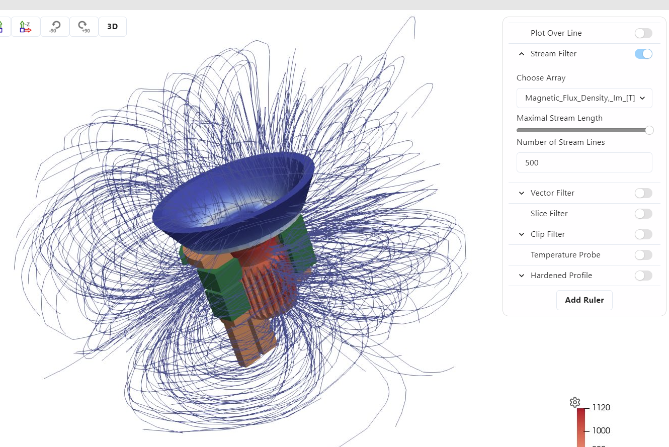
Stream Filter

Stream filter shows the magnetic field. You can choose if it displays the real or imaginary values of the field, the maximum stream length (how far from the center of the air box to the sides the stream lines go – the bigger the length, the more of the air box space the stream lines will occupy), and the number of stream lines – the more lines, the more condensed you will see the field.

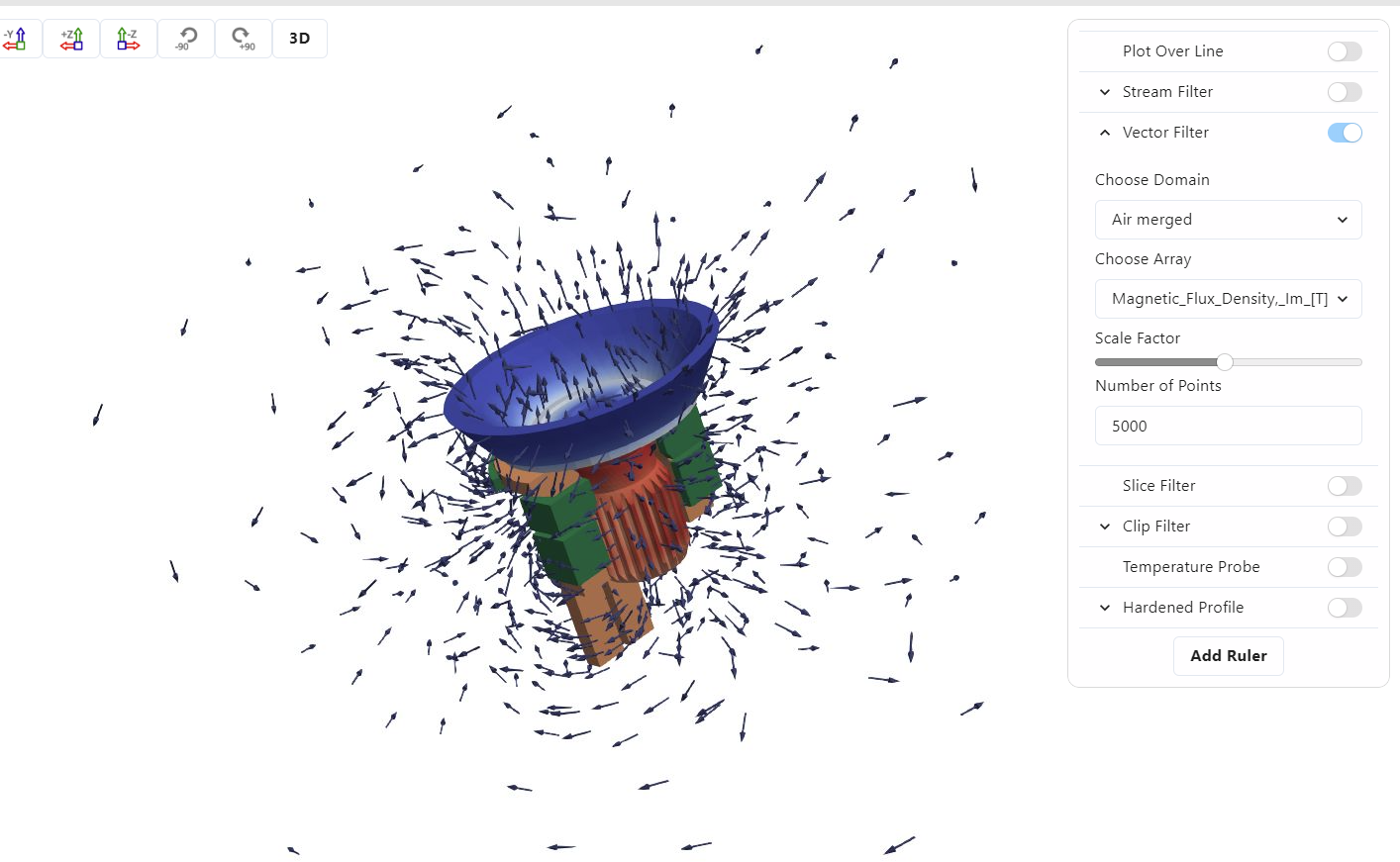
Vector Filter

The Vector Filter is quite similar to Stream Filter – but instead of lines it shows vectors.

For this filter you can also choose the domain – any of the solids. Each domain can have different results displayed with the vectors, for example, the air domain will have magnetic flux density, however, the inductor will have current density.

You can choose the vector scale factor – how big the arrows will be displayed, as well as the number of points – the more points, the more arrows you will see.

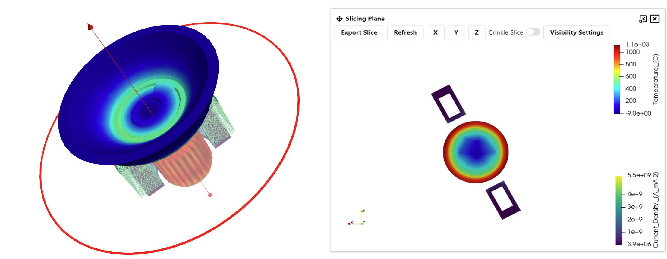
Slice Filter

The slice filter creates a 2D image of the geometry that is on the selected plane. There will be a popup window with the available options.

You can select the plane to be on a specific axis, by clicking X, Y or Z or you can manually move the plane by dragging it with your mouse. After the modifications you can click Refresh to see the slice.

You can also save the slice image by clicking ‘Export slice’, crinkle the slice or choose visibility settings.

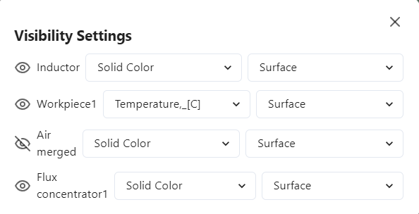
In the visibility settings you can choose which solids and how appear in the slice.

Clip Filter

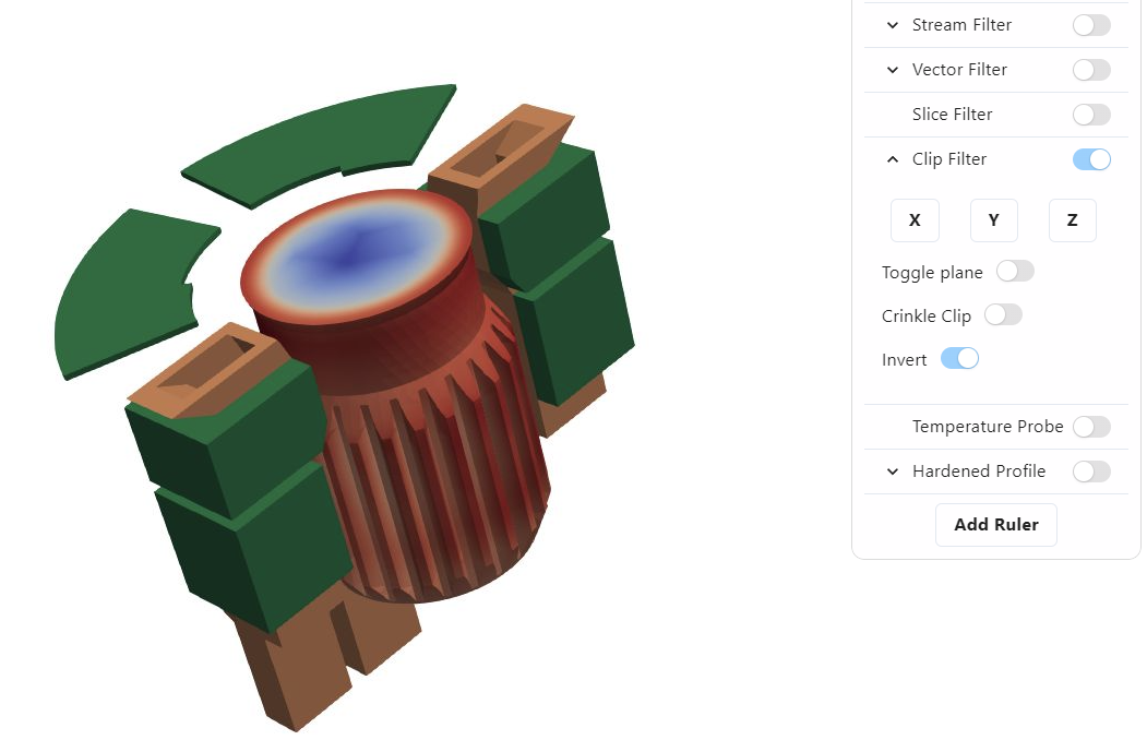
This filter cuts the geometry. You can choose the plane (X, Y or Z) or manually drag it. You can turn it on or off by the toggle.

You can also crinkle the clip and invert it.

Temperature Probe

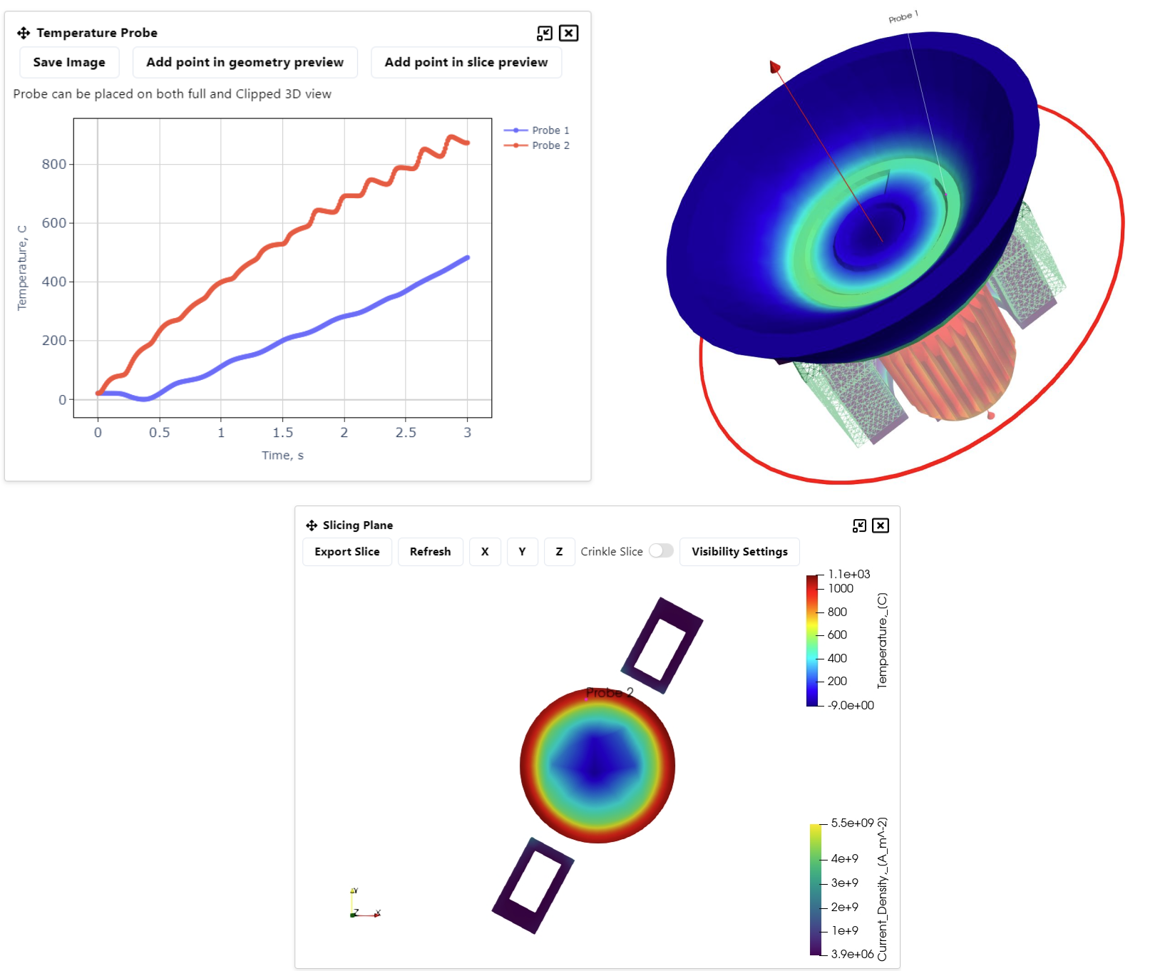
A temperature probe allows you to view temperature changes in a specific point (or mesh cell if the geometry has complex motion) over the whole simulation time.

It can be used on a full 3D geometry or on a clip. It can also be used in a slice.

• In 3D, you need to click ‘Add point in geometry preview’ in the probe popup window and then select a point on the geometry. The selection will snap to the closest mesh crossing point or the closest mesh cell and then display the plot in the popup window.

• For a slice, choose the ‘Add point in slice preview’ option. If you have not opened the slice yet, this option will automatically open the slice filter for you and you just have to select the point in the popup window.

Similarily to plot over line – the created probes can be toggled visible or invisible by clicking on their names in the temperature probe popup window. They can be deleted by clicking the trash icon next to their name when they appear under all the filters on the right side.

Hardened Profile

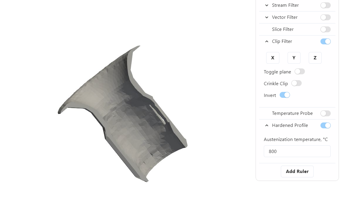
The hardened profile filter allows you to see where on the workpiece the specified Austenization temperature has been reached. By default it is set to 800 degrees Celsius.

The hardened area shows up gray in the visualization view. You can turn off the visibility for the geometry objects and use the clip filter to better see the profile.

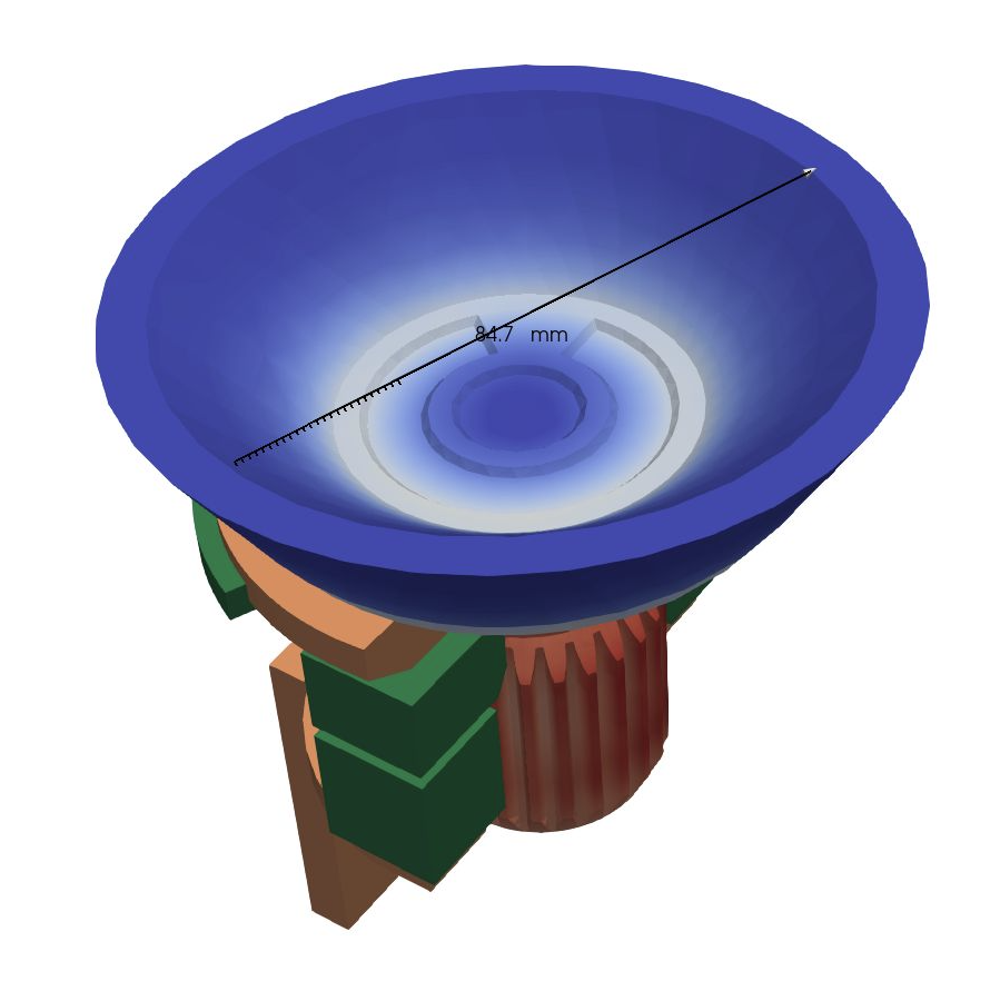
Ruler

When you press ‘Add ruler’, you will see a line with measurements appear on screen. This ruler will also appear on the right side under the filters.

From there you can toggle its visibility, delete it and toggle snap to point.

Snap to point means that when you drag the ends of the ruler, they will snap to the closest mesh element.

Automatic Results

The results in CENOS Results Viewer have been divided into multiple tabs.

Each tab has a preset of enabled filters and results that are opened automatically, to ease the viewing process.

• HEATING: This is the tab that is opened first when the results load after the simulation. It is also the tab from which the previous sections on results and filters have been shown.
• MAGNETIC FIELD: This tab automatically has Stream filter enabled to show the magnetic field lines.
• WORKPIECE: This tab has only workpiece visible, it also has the Slice filter enabled automatically.
• INDUCTOR & FLUX CONCENTRATORS: This tab only shows the inductor and flux concentrators if they are present. It has automatically set current density to the inductor.
• PERFORMANCE PLOTS: This tab shows different plots.

Performance Plots

The last tab in CENOS Results Viewer contains all kinds of performance plots. When you open it, the first plot that opens is the Active Power plot:

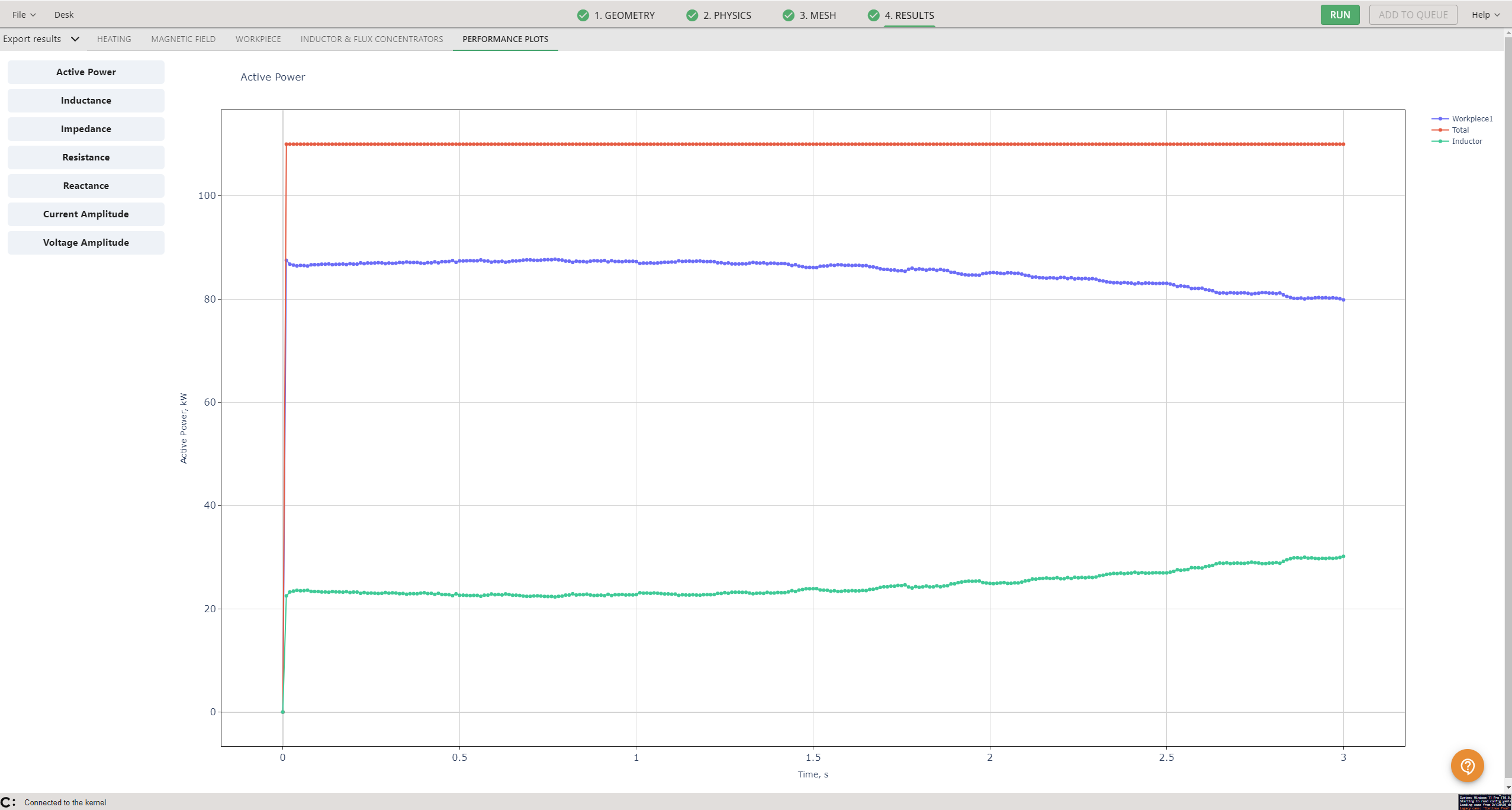
On the left side you can select a different plot to view. The plots are:

• Active Power
• Inductance
• Impedance
• Resistance
• Reactance
• Cuurent Amplitude
• Voltage Amplitude
• Connective Power Loss
• Radiative Power Loss

Export Results

The EXPORT RESULTS dropdown has multiple options:

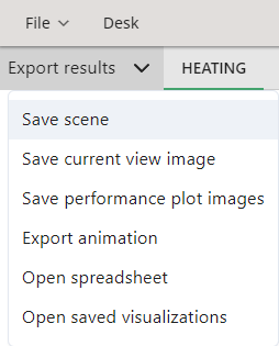
• Save scene: saves the current applied filters, colors etc.
• Save current view image: saves the current 3D view to the case results folder.
• Save performance plots images: saves the performance plots as images to the case results folder.
• Export animation: saves the simulation animation as a .gif file to the case results folder.
• Open spreadsheet: opens the results .csv file.
• Open saved visualizations

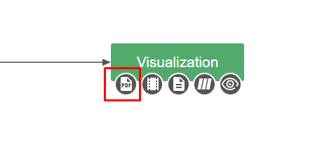
You can also generate a pdf report by going back to the DESK view and clicking on the pdf button under Visualization: