Defining motion

Movement is an important part for a lot of induction heating systems, as translational or rotational movement helps to heat/harden the specific part uniformly and efficiently. To accurately simulate such processes, you need to take into account the respective types and speeds of the movement present in your system.

In this article we are going to take a look at how movement can be defined in CENOS, what are the requirements for movement and what limitations are currently present with such setup.

Motion in CENOS​

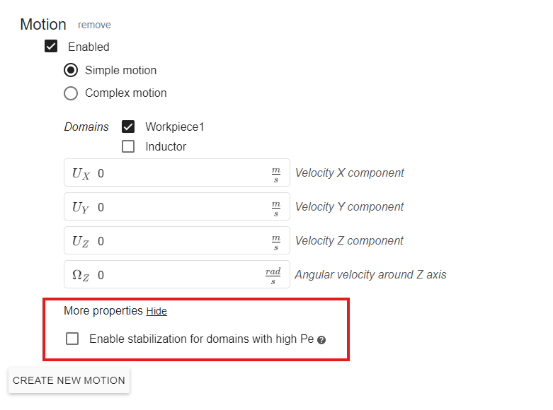
CENOS supports both translational (scanning) and rotational (single-shot) movement. To define motion in your simulation, go to the Motion tab in the PHYSICS section and click CREATE NEW MOTION.

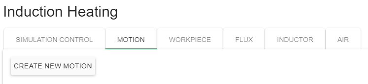
Select the type of motion, which part you want to move, in which direction, and with what speed, and CENOS will do the rest!

Types of Motion​

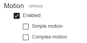
When defining Motion, you will notice that there are 2 options to choose from – Simple Motion and Complex Motion.

Note: When using CENOS: Wireless Charging, we strongly recommend only using Complex Motion, as usually Wireless Charging systems geometrically are not suitable for Simple motion.

Simple Motion​

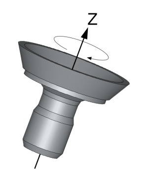
This option allows you to simulate motion for axially symmetrical or continuous workpieces.

Some examples would include:

As you can see, Simple Motion can be applied to systems where it can be assumed that the geometry is not moving. This can be very useful for completely symmetrical part rotation or modelling of continuous feed of material through the system.

Note:

1. Use Simple Motion if it is possible, as it calculates a lot faster than Complex Motion.
2. Simple Motion can be set only for the workpiece – if you set it to the inductor or flux concentrators, you will not see any temperature changes.
3. When setting up the direction and speed for Simple Motion, you should think of where you would like the heat to travel – this is often (specifically in translation cases) the opposite direction from what you would set for Complex Motion.

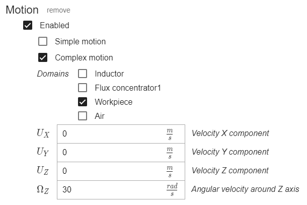
Complex Motion​

If Simple Motion is not applicable to your case, you need to use Complex Motion.

For parts with splines, teeth, holes, gaps and other kinds on unsymmetrical details an actual motion needs to be simulated. Complex Motion enables you to move the respective parts in your system.

Note: Make sure that the calculation time step is small enough to capture the rotation smoothly! No more than 30 deg turn in one time step!

Limitations​

Even though the Movement definition is easy to use, there are still some things to keep in mind when defining movement in CENOS.

Rotation axis​

Rotation currently is limited only around the Z axis, so be sure that your rotational system is positioned around the Z axis!

Stabilization

In cases when you are using a plastic, epoxide or polymeric material of some kind and want to use very fast simple motion speed, you need to enable stabilization to get accurate results.

Stabilization techniques are required in simulations when the heat transfer Péclet number (Pe) is much greater than 1 (Pe >> 1). The Péclet number describes the relative importance of advective (convective) transport compared to diffusive transport.

When advective transport – which is associated with material motion or convection velocity – is significantly larger than diffusive transport – which is governed by thermal conductivity – the Péclet number becomes large.

In such cases, numerical simulations may become unstable.

This instability typically appears as:

• Non-physical temperature distributions
• Oscillations in the temperature field
• Difficulties with solver convergence

Definition of the Péclet Number

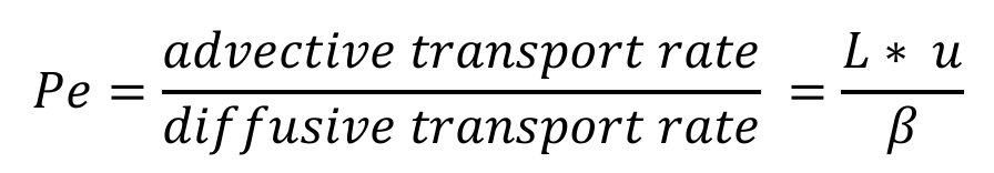
where the thermal diffusivity 𝛽 is defined as

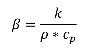
Parameters:

• 𝐿— characteristic mesh cell size
• 𝑢— material or flow velocity
• 𝑘— thermal conductivity
• 𝜌— material density
• 𝑐𝑝— specific heat capacity

Example case

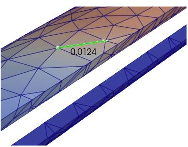
• Mesh cell size (in picture) ~0.01 m,
• Velocity – 0.03 m/sec,
• k – 0.3 W/mK,
• cp-1150 J/kg*K,
• rho-1900 kg/m3

If we calculate Pe number it is:

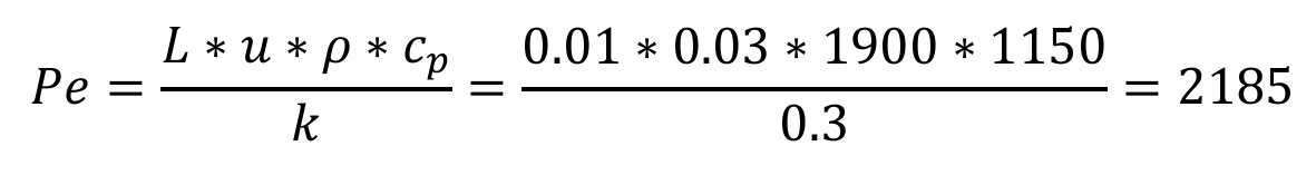
In this case Pe>> 1 which will cause unstable simulation.

Determining the Stabilization Coefficient

To reduce numerical problems when the Péclet number is very high (Pe >> 1), a stabilization term with a parameter 𝛼 is added to the governing equations.

To determine a suitable value for 𝛼:

1. Start with a value in the range 0.1–0.2
2. If numerical instabilities persist, gradually increase the value until stable and physically realistic results are obtained.

For similar simulation setups – that is, cases with comparable geometry, motion speeds, mesh sizes, and material properties – the required stabilization coefficient will typically be similar.